
In a previous post (here), we saw how we can determine sample size for obtaining, with assurance, a precise interaction contrast estimate. In that post we considered a 2 x 2 factorial design. In this post, I will extend the discussion to the mixed model case. That is, we will consider sample size planning for a precise interaction estimate in case of a design with 2 fixed factors and two random factors: participant and stimulus (item). (A pdf version of this post can be found here: view pdf. )
In order to keep things relatively simple, we will focus on a design where both participants and items are nested under condition. So, each treatment condition has a unique sample of participants and items. We will call this design the both-within-condition design (see, for instance, Westfall et al. 2014, for detailed descriptions of this design). We will analyse the 2 x 2 factorial design as a single factor design (the factor has a = 4 levels) and formulate an interaction contrast.
Let’s start with p participants and q stimuli. We randomly assign n= p/a participants and m = q/a stimuli to each of the a treatment levels. The ANOVA table for the design is presented in Table 1.

Obtaining an apropriate error term
UNIANOVA score BY cond pp ss
/RANDOM=pp ss
/METHOD=SSTYPE(3)
/INTERCEPT=INCLUDE
/CRITERIA=ALPHA(0.05)
/DESIGN=cond pp WITHIN cond ss WITHIN cond
/CONTRAST(cond) = SPECIAL(1, -1, -1, 1).
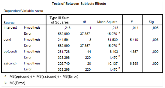 |
| Figure 1: SPSS GLM ANOVA output |
Take a look at Table 1 and focus on the Participant row. The expected Mean Square (EMS) associated with Participant is  . Now, suppose that due to some freak accident of nature there are no differences in the mean scores (averaged of stimuli) of each participant. In that case,
  . This means that under these circumstances the expected mean square associated with participants is simply an estimate of the error variance with
  degrees of freedom, because
  , if . Of course, the other estimate of the Error variance is MSError and this estimate is based on
  degrees of freedom. The logic of the F-test is that under the null-hypothesis, in our case that , the ratio of these two estimates of the error variance follows an F-distribution with and degrees of freedom.
Now focus on the Treatment row in Table 1. The expected mean square associated with Treatment equals  . If we now suppose that there is no difference between the treatment means, that is
  , MSTreatment does not estimate
  , but
, but  . Note that no other source of variance has an expected mean square that is equal to the latter figure. That is, in contrast to our test of the Participant factor, where under the null-hypotheses two Mean Squares estimate the error variance, i.e. MSParticipant and MSError, no mean square is available to form an F-ratio to test the Treatment effect.
But a linear combination of MSParticipant, MSStimulus and MSError, does provide an estimate with expected value . Namely, the sum of the participant and stimulus mean squares minus mean square error: ![[m\sigma^2_p + \sigma^2_e] + [m\sigma^2_s + \sigma^2_e] - [\sigma^2_e] = m\sigma^2_p + n\sigma^2_s + \sigma^2_e](https://small-s.science/wp-content/ql-cache/quicklatex.com-9cd6bb15506816413e74641fee23cf13_l3.png "Rendered by QuickLaTeX.com") . It is exactly this linear combination of mean squares that is used in the F-ratio to obtain an error term against which to test the Treatment effect in Figure 1:
. It is exactly this linear combination of mean squares that is used in the F-ratio to obtain an error term against which to test the Treatment effect in Figure 1:  . We will also use this figure to obtain the variance (and standard error) of our contrast estimate.
Degrees of freedom
If you take a closer look at Figure 1, in particular the degrees of freedom column, you will notice that the degrees of freedom associated with the error term that is used to test the Treatment effect is a fractional number and not a nice round number that you would expect to get if you only consider the degrees of freedom in Table 1. The cause of this fractional number is that we cannot simply use the degrees of freedom of the mean square used to test the treatment effect, because that mean square does not exist. Indeed, we had to combine three mean squares in order to obtain an estimate of the error term for the Treatment effect. The consequence of this is that we will have to use an approximation of the degrees of freedom associated with that error term.
SPSS (and my precision app) use the Satterthwaite procedure to approximate the degrees of freedom of the error term. That approximation is as follows (notice that the numerator is equal to the linear combination of mean squares used to obtain the error term).
![\[df=\frac{(MSp+MSs-MSe)^{2}}{\frac{MSp^{2}}{df_{p}}+\frac{MSs^{2}}{df_{s}}+\frac{MSe^{2}}{df_{e}}}.\]](https://small-s.science/wp-content/ql-cache/quicklatex.com-13f753be88a6e13890953c2465e22a05_l3.png "Rendered by QuickLaTeX.com")
Thus, using the results in Figure 1.
MSp = 6.403
MSs = 10.137
MSe = 1.470
dfp = 44
dfs = 20
dfe = 220
df = (MSp + MSs - MSe)^2 / (MSp^2/dfp + MSs^2/dfs + MSe^2/dfe)
df
## [1] 37.35559
The margin of error of a contrast estimate
Now that we have obtained the error variance of a treatment effect by using a linear combination of mean squares and a Satterthwaite approximation of the degrees of freedom we are able to figure out the margin of error (MOE) of our contrast estimate. Just as in the simple between subjects design we discussed previously we obtain MOE by multiplying the standard error of the estimate with a critical value of t. The critical value of t is the .975 quantile of the central t-distribution with the Satterthwaite approximated degrees of freedom (if you are looking for something other than a 95% confidence interval, you will have to use another critical value, of course). The following code gives the critical value of t for a 95% confidence interval (change the value of C if you want something other than a 95% interval).
C = .95
alpha = 1 - C
critT = qt(1 - alpha/2, df)
critT
## [1] 2.025542
The standard error of the contrast estimate  can be obtained as follows.
![\[\hat{\sigma}_{\hat{\psi}}=\sqrt{\sum c_{i}^{2}\hat{\sigma}_{\bar{X},Rel}^{2}},\]](https://small-s.science/wp-content/ql-cache/quicklatex.com-489e315828278a9811848f3ce71bf10f_l3.png "Rendered by QuickLaTeX.com")
where I have used the symbol  to refer to the relative error variance of the treatment mean (which in this design is equal to the absolute error variance, but that’s another story), and
  refers to the contrast weight of treatment mean i. The relative error variance of the treatment mean is obtained by dividing the error variance that is used to test the treatment effect by the total number of observations in each treament,
  . Thus, using the results in Figure 1.
![\[\hat{\sigma}_{\bar{X},Rel}^{2}=\frac{MS_{p}+MS_{s}-MS_{e}}{nm}=\frac{15.07}{72}=0.2093.\]](https://small-s.science/wp-content/ql-cache/quicklatex.com-0d81fe2ec65ea2c26c84682713e499bf_l3.png "Rendered by QuickLaTeX.com")
If we want to estimate an interaction contrast for the 2 x 2 design, we may, for example, specify contrasts weights  . Let’s use the results in Figure 1 to calculate what MOE is for this particular contrast.
#sample sizes per treatment
n = 12
m = 6

#obtained mean squares (see Figure 1):
MSp = 6.403
MSs = 10.137
MSe = 1.470

#Relative error variance:
VarT = (MSp + MSs - MSe) / (n*m)

#contrast weights:
weights = c(1, -1, -1, 1)

#standard error of contrast estimate
SEcontrast = sqrt(sum(weights^2)*VarT)

#Satterthwaite degrees of freedom:
dfp = 44
dfs = 20
dfe = 220
df = (MSp + MSs - MSe)^2 / (MSp^2/dfp + MSs^2/dfs + MSe^2/dfe)

#critical T
critT = qt(.975, df)

#Margin of Error
MOE = critT * SEcontrast

SEcontrast; MOE
## [1] 0.9149985
## [1] 1.853368
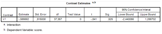
SPSS GLM Univariate uses the wrong standard error for a mixed model contrast estimate
Even though SPSS GLM Univariate allows you to specify a mixed model design and tests the treatment effect with a linear combination of mean squares, the procedure does not use the correct error variance if you want to estimate the value of a contrast (using the CONTRAST subcommand), it uses MSError instead. In our example, then, SPSS uses an error variance that is an order of magnitude smaller than the correct error variance:  , with 220 degrees of freedom and not
  , with 37.357 (see Figure 1). The consequence of this is, of course, that the 95% CI is much narrower than it should be.
Running the syntax above Figure 1 gives the output in Figure 2. The results can be reproduced as follows. The standard error of the contrast is the result of  , the critical value of t is the .975 quantile of the central t distribution with
  , which equals
  . The value of MOE is therefore
  . With a contrast estimate of
  , the 95% CI equals
 ![-0.587 \pm 0.5633 = [-1.1503, -0.0237]](https://small-s.science/wp-content/ql-cache/quicklatex.com-ea5612615f1baf096374644a223d775f_l3.png "Rendered by QuickLaTeX.com") . In comparison, using the correct value of MOE gives us
. In comparison, using the correct value of MOE gives us ![[−2.4404, 1.2664]](https://small-s.science/wp-content/ql-cache/quicklatex.com-ef97651e8790dc304790e8a8724ebed7_l3.png "Rendered by QuickLaTeX.com") .
.
 |
| Figure 2: SPSS GLM Univariate Contrasts Output |
MIXED score BY cond
/CRITERIA=CIN(95) MXITER(100) MXSTEP(10) SCORING(1)
SINGULAR(0.000000000001) HCONVERGE(0, ABSOLUTE)
LCONVERGE(0, ABSOLUTE) PCONVERGE(0.000001, ABSOLUTE)
/FIXED= cond | SSTYPE(3)
/METHOD=REML
/TEST= 'interaction' cond 1 -1 -1 1
/RANDOM=INTERCEPT | SUBJECT(pp) COVTYPE(VC)
/RANDOM=INTERCEPT | SUBJECT(ss) COVTYPE(VC).
 |
| Figure 3: Contrast Estimate SPSS Mixed |
Planning for precision
Even though the result in Figure 3 is hard to interpret without substantive detail (the data are made up) it is clear that the precision of the estimate is, well, suboptimal. As an indication: the estimated within treatment standard deviaion is about 1.74, so the estimated difference between differences (interaction) is close to a value of Cohen’s d of  , approximate 95% CI
 ![[-1.40, 0.73]](https://small-s.science/wp-content/ql-cache/quicklatex.com-867264624a612f401b2c1cea536372a9_l3.png "Rendered by QuickLaTeX.com") , which according to the rules of thumb is a medium negative effect, but consistent with anytihing from a huge negative effect to a large positive effect in the population, as the approximate CI shows. (I have divided the point estimate and the confidence interval in Figure 2 by 1.74, to obtain Cohen’s d and an approximate confidence interval). Clearly, then, our precision can be optimized.
, which according to the rules of thumb is a medium negative effect, but consistent with anytihing from a huge negative effect to a large positive effect in the population, as the approximate CI shows. (I have divided the point estimate and the confidence interval in Figure 2 by 1.74, to obtain Cohen’s d and an approximate confidence interval). Clearly, then, our precision can be optimized.
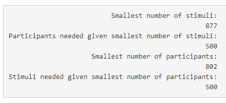
Suppose that you are very fond of the both-within-condition design (BwC-design) and you plan to use it again in a replication study, You could of courseopt for a design with better expected precision, but based on the data and estimates at hand, that involves a lot of assumptions, but I will show you how you can do it in one of the next posts. If you plan for precision using the BwC-design, you need the following ingrediënts.
1. A figure for your target MOE. Let’s set target MOE to .40.
2. A specification of the percentage of assurance. Let’s say we want 80% assurance that target MOE will not exceed .40.
3. Estimates (or guesstimates) of the person variance  , the stimulus variance
  , and the error variance . We will have a look in the next section.
4. Functions for calculating the relative error variance, degrees of freedom, MOE and determining the required sample sizes for Participants and Stimuli. These are all present in the Precision App, so I will use the application, but I will show how the results of the sample sizes relate to the information above.
Obtaining estimates of the variance components
We need to specify the values of three variance components. These variance components can be estimated on the basis of the mean squares and sample sizes obtained with SPSS GLM Univariate, we can use SPSS MIXED to obtain direct estimates or any other way to estimate variance components, such as GLM VARCOMPS (which has several estimation procedures). I like to use SPSS MIXED or LME4. and not a dedicated program for variance components, because most of the times the main purpose of the analysis I am doing is obtaining contrast estimate or F-tests, so most of the times variance components estimates are a handy by-product of my main analysis. For demonstrative purposes, I will show how it can be done with the GLM univariate output and I will show how the results match those of SPSS MIXED.
Take a look at Figure 1. The estimate of is simply MS(Error) = 1.47. For obtaining an estimate for the variance component associated with participants, we set the obtained mean square equal to the expected mean square (see Table 1). Thus,  . Rearranging and using 1.47 as an estimate for leads to
  . Likewise, the estimate for
  . Thus, our estimates are
  ,
,  , and
, and  .
.
In order to obtain direct estimates you can use SPSS Mixed (or GLM Varcomps, or whatever you like). If you run the SPSS syntax in Figure 3, you will find estimates of the variance components under the heading Covariance Parameters in your SPSS output. See Figure 4. Note that the standard errors are pretty large, so the point estimates are not very precise. But since it is the only information we have, we will consider the point estimates to be the best we have.
 |
| Figure 4: Variance components estimates |
Getting sample sizes with the Precision application
(Note: it is not necessary to fill it in in contrast 3). , for assurance the value .80 and the values ,
  , and
, and  for, respectively, Residual variance, Participant intercept variance and Stimulus intercept variance. Fill in the value 0 for all the other variances. See Figure 5.
 |
| Figure 5: Setting values in the Precision App. |
 |
| Figure 6a: Output for planning target MOE = 0.40 |
 |
| Figure 6b: Outpur for planning target MOE = 0.50 |
 , to refer to the residual variance in the BwC-design, we can say
  . Normally, the precision app sums these two components to get a value for the residual variance in the BwC-design, and you will obviously get the same result if you specify the residual variance as the sum and the participant-by-stimulus variance as 0. Likewise,
  , and
, and  , where
  and
and  are the variances associated with the interaction of treatment and participant and treatment and stimulus, respectively.
Checking the sample size suggestions using what we know
 , and there is 80% assurance that MOE will not exceed
  . Note, again, that the assurance MOE is somewhat larger than target MOE, because a sample of 804 participants requires a sample of more than 500 stimuli to get the target MOE with 80% assurance and 500 stimuli is the maximum number of stimuli the app considers when minimizing the number of participants.
 |
| Figure 7: Expected and Assurance MOE for the interaction contrast (contrast 3) using 804 participants and 500 stimuli |

 ,
,  ,
,  ,
,  ,
,  , and
, and  . The Satterthwaite degrees of freedom are
  . The standard error of the contrast equals
  . The critical value for t equals
  . Expected MOE is, therefore,
  (the tiny difference with the results from the app is due to rounding errors).
 -distribution. That is, we assume with assurance
  , that the quantile of the sampling distribution of the relative error error variance is
  . Now, the degrees of freedom are
  , the assurance
  , and the .80 quantile of with 1092.66 degrees of freedom equals
  . Since the relative error variance equals
  , the .80 quantile of the error variance equals
  . And this means that assurance MOE equals
  . Again, the difference with the results from the Precision App are due to rounding error.