Comparing the quantiles of two groups

Comparing the quantiles of two groups provides information that is lost by simply looking at means or medians. This post shows how to do that.

Traditionally,  the comparison of two groups focuses on comparing means or medians.  But, as Wilcox (2012) explains, there are many more features of the distributions of two groups that we may compare in order to shed light on how the groups differ. An interesting approach is to estimate the difference between the quantiles of the two groups.  Wilcox (2012, pp. 138-150) shows us an approach that is based on the shift function. The procedure boils down to estimating the quantiles of both groups, and plotting the quantiles of the first group against the difference between the quantiles.

In order to aid in comparing the quantiles of the groups, I’ve created a function for R that can be used for plotting the comparison between the two groups. The functions uses the ggplot2 package and the WRS package (that can be found here: WRS: A package of R.R. Wilcox’ robust statistics functions version 0.24 from R-Forge (rdrr.io)) ; see also: Installation of WRS package (Wilcox’ Robust Statistics) | R-bloggers (r-bloggers.com).).

library(WRS)
library(ggplot2)

plotSband <- function(x, y, x.name = "Control") {
  x <- sort(x[!is.na(x)])
  y <- sort(y[!is.na(y)]) 
  qhat <- 1:length(x)/length(x)
  idx.y <- floor(qhat*length(y) + .5)
  idx.y[idx.y <= 0] <- 1
  idx.y[idx.y > length(y)] <- length(y)
  
  delta <- y[idx.y] - x
  
  cis <- WRS::sband(x, y, plotit=F)$m[, c(2, 3)]
  
  check.missing <- apply(cis, 2, function(x) sum(is.na(x)))
  if (sum(check.missing == length(x)) > 1) {
    stop("All CI limits equal to - or + Infinity")
  }
  ylims <- c(min(cis[!is.na(cis[,1]), 1]) - .50, 
             max(cis[!is.na(cis[,2]), 2]) + .50)
  
  cis[is.na(cis[, 1]), 1] <- ylims[1]*5
  cis[is.na(cis[, 2]), 2] <- ylims[2]*5
  
  thePlot <- ggplot(mapping = aes(x)) + 
    xlab(x.name) + 
    geom_smooth(aes(x = x, y = delta), se = F, col="blue") + 
    ylab("Delta") +
    geom_point(aes(x = quantile(x, c(.25, .50, .75)), 
                   y = rep(ylims[1], 3)), pch=c(3, 2, 3), size=2) +
    geom_ribbon(aes(ymin = cis[,1], ymax = cis[,2]), alpha=.20) + 
    coord_cartesian(ylim = ylims)
  suppressMessages(print(thePlot))
}

Let’s look at an example. Figure 1 presents data from an experiment investigating the persuasive effect of narratives on intentions of adopting a healthy lifestyle (see for details Boeijinga, Hoeken, and Sanders (2017)). The plotted data are the differences in intention between the quantiles of a group of participants who read a narrative focusing on risk-perception (detailing the risks of unhealthy behavior) and a group of participants who read a narrative focusing on action-planning (here called the control group), focusing on how the healthy behavior may actually be implemented by the participant.

Comparing the quantiles of two groups
Figure 1. Output from the plotSband-function

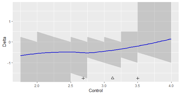
Figure 1 shows the following. The triangle is the median of the data in the control group, and the plusses the .25th and .75th quantiles. The shaded regions define the simultaneous 95% confidence intervals for the differences between the quantiles of the two groups. Here, these regions appear quite ragged, because of the discrete nature of the data. For values below 2.5 and above 3.5, the limits (respectively the lower and upper limits of the 95% CI’S) equal infinity, so these values extend beyond the limits of the y-axis. (The sband function returns NA for these limits). The smoothed-regression line should help interpret the general trend.

How can we interpret Figure 1? First of all, if you think that it is important to look at statistical significance, note that none of the 95% intervals exclude zero, so none of the differences reach the traditional significance at the .05 level. As we can see, none of them exclude differences as large as -0.50 as well, so we should not be tempted to conclude that because zero is in the interval that we should adopt zero as the point-estimate. For instance, if we look at x = 2.5, we see that the 95% CI equlas [-1.5, 0.0], the value zero is included interval, but so is the value -1.5. It would be unlogical to conclude that zero is our best estimate if so many values are included in the interval.

The loess-regression line suggests that the differences in quantiles between the two groups of the narrative is relatively steady for the lower quantiles of the distribution (up to the x = 3.0, or so; or at least below the median), but for quantiles larger than the median the effect gets smaller and smaller until the regression line crosses zero at the value x = 3.75. This value is approximately the .88 quantile of the distribution of the scores in the control condition (this is not shown in the graph).

The values on the y-axis are the differences between the quantiles. A negative delta means that the quantile of the control condition has a larger value than the corresponding quantile in the experimental condition. The results therefore suggest that participants in the control condition with a relatively low intention score, would have scored even lower in the other condition. To give some perspective: expressed in the number of standard deviations of the intention scores in the control group a delta of -0.50 corresponds to a 0.8 SD difference.

Note however, that due to the limited number of observations in the experiment, the uncertainty about the direction of the effect is very large, especially in the tails of the distribution (roughly below the .25 and above the .75 quantile). So, even though the data suggest that Action Planning leads to more positive intentions, especially for the lower quantiles, but still considerably for the .75 quantile, a (much) larger dataset is needed to obtain more convincing evidence for this pattern.

A confidence interval for the correlation coefficient

A confidence interval for the  population correlation coefficient \rho can be obtained with the Fisher-r-to-z transformation.   The steps are as follows.

  1. Transform r to a standard normal deviate Z
    Z_{xy} = \frac{1}{2}ln\left(\frac{1 + r}{1  –  r}\right), \tag{1}
    which is equal to:
    Z_{xy} = arctanh(r). \tag{2}
  2. Determine the standard error for Z:
    s_Z = \sqrt\frac{1}{N  –  3}. \tag{3}
  3. Calculate the Margin of Error (MoE) for Z:
    MOE_Z = 1.96*s_z. \tag{4}
  4. Add to and substract MoE  from Z to obtain a 95% Confidence Interval for Z.
  5. Transform the upper and lower limits of the CI for Z to obtain the corresponding limits for \rho, using:
    r_Z = \frac{e^{2Z} –  1}{e^{2Z} + 1}, \tag{4}
    which is equal to:
    r_Z = tanh(Z). \tag{5}

The following R-code does all the work:

conf.int.rho <- function(r, N) {
lims.rho =  tanh(atanh(r) + c(qnorm(.025), 
			qnorm(.975)) * sqrt(1/(N - 3)))
return(lims.rho)
}

So, if you have r = .50 and N = .50, just run the above function in R to obtain a confidence interval for the correlation coefficient. 

conf.int.rho(.50, 50)

## [1] 0.2574879 0.6832563


Linear Trend Analysis with R and SPSS

This is an introduction to contrast analysis for estimating the  linear trend among condition means with R and SPSS . The tutorial focuses on obtaining point and confidence intervals.  The contents of this introduction is based on Maxwell, Delaney, and Kelley (2017) and Rosenthal, Rosnow, and Rubin (2000). I have taken the (invented) data from Haans (2018). The estimation perspective to statistical analysis is aimed at obtaining point and interval estimates of effect sizes. Here, I will use the frequentist perspective of obtaining a point estimate and a 95% Confidence Interval of the relevant effect size. For linear trend analysis, the relevant effect size is the slope coefficient of the linear trend, so, the purpose of the analysis is to estimate the value of the slope and the 95% confidence interval of the estimate. We will use contrast analysis to obtain the relevant data.

[Note: A pdf-file that differs only slightly from this blogpost can be found on my Researchgate page: here; I suggest Haans (2018) for an easy to follow introduction to contrast analysis, which should really help understanding what is being said below].

The references cited above are clear about how to construct contrast coefficients (lambda coefficients) for linear trends (and non-linear trends for that matter) that can be used to perform a significance test for the null-hypothesis that the slope equals zero. Maxwell, Delaney, and Kelley (2017) describe how to obtain a confidence interval for the slope and make clear that to obtain interpretable results from the software we use, we should consider how the linear trend contrast values are scaled. That is, standard software (like SPSS) gives us a point estimate and a confidence interval for the contrast estimate, but depending on how the coefficients are scaled, these estimates are not necessarily interpretable in terms of the slope of the linear trend, as I will make clear
momentarily.

So our goal of the data-analysis is to obtain a point and interval estimate of the slope of the linear trend and the purpose of this contribution is to show how to obtain output that is interpretable as such.

Continue reading “Linear Trend Analysis with R and SPSS”

Planning for Precise Contrast Estimates: Introduction and Tutorial (Preprint)

I just finished a preprint of an introduction and tutorial to sample size planning for precision of contrast estimates. The tutorial focuses on single factor between and within subjects designs, and mixed factorial designs with one within and one between factor. The tutorial contains R-code for sample size planning in these designs.

The preprint is availabe on researchgate: Click (but I am just as happy to send it to you if you like; just let me know).

Contrast analysis with R: Tutorial for factorial mixed designs

In this tutorial I will show how contrast estimates can be obtained with R. Previous posts focused on the analyses in factorial between and within designs, now I will focus on a mixed design with one between participants factor and one within participants factor. I will discuss how to obtain an estimate of an interaction contrast using a dataset provided by Haans (2018).

I will illustrate two approaches, the first approach is to use transformed scores in combination with one-sample t-tests, and the other approach uses the univariate mixed model approach. As was explained in the previous tutorial, the first approach tests each contrast against it’s own error variance, whereas in the mixed model approach a common error variance is used (which requires statistical assumptions that will probably not apply in practice; the advantage of the mixed model approach, if its assumptions apply,  is that the Margin of Error of the contrast estimate is somewhat smaller).

Again, our example is taken from Haans (2018; see also this post. It considers the effect of students’ seating distance from the teacher and the educational performance of the students: the closer to the teacher the student is seated, the higher the performance. A “theory “explaining the effect is that the effect is mainly caused by the teacher having decreased levels of eye contact with the students sitting farther to the back in the lecture hall. To test that theory, a experiment was conducted with N = 9 participants in a factorial mixed design (also called a split-plot design), with two fixed factors: the between participants Sunglasses (with or without), and the within participants factor Location (row 1 through row 4). The dependent variable was the score on a 10-item questionnaire about the contents of the lecture. So, we have a 2 by 4  mixed factorial design, with n = 9 participants in each combination of the factor levels.

We will again focus on obtaining an interaction contrast: we will estimate the extent to which the difference between the mean retention score on the first row and those on the other rows differs between the conditions with and without sunglasses.

Continue reading “Contrast analysis with R: Tutorial for factorial mixed designs”

Planning with assurance, with assurance

Planning for precision requires that we choose a target Margin of Error (MoE; see this post for an introduction to the basic concepts) and a value for assurance, the probability that MoE will not exceed our target MoE.  What your exact target MoE will be depends on your research goals, of course.

Cumming and Calin-Jageman (2017, p. 277) propose a strategy for determining target MoE. You can use this strategy if your research goal is to provide strong evidence that the effect size is non-zero. The strategy is to divide the expected value of the difference by two, and to use that result as your target MoE.

Let’s restrict our attention to the comparison of two means. If the expected difference between the two means is Cohens’s d = .80, the proposed strategy is to set your target MoE at f = .40, which means that your target MoE is set at .40 standard deviations. If you plan for this value of target MoE with 80% assurance, the recommended sample size is n = 55 participants per group. These results are guaranteed to be true, if it is known for a fact that Cohen’s d is .80 and all statistical assumptions apply.

But it is generally not known for a fact that Cohen’s d has a particular value and so we need to answer a non-trivial question: what effect size can we reasonably expect? And, how can we have assurance that the MoE will not exceed half the unknown true effect size? One of the many options we have for answering this question is to conduct a pilot study, estimate the plausible values of the effect size and use these values for sample size planning.  I will describe a strategy that basically mirrors the sample size planning for power approach described by Anderson, Kelley, and Maxwell (2017).

The procedure is as follows. In order to plan with approximately 80% assurance, estimate on the basis of your pilot the 80% confidence interval for the population effect size and use half the value of the lower limit for sample size planning with 90% assurance. This will give you 81% assurance that assurance MoE is no larger than half the unknown true effect size.

The logic of planning with assurance, with assurance

There are two “problems” we need to consider when estimating the true effect size. The first problem is that there is at least 50% probability of obtaining an overestimate of the true effect size. If that happens, and we take the point estimate of the effect size as input for sample size planning, what we “believe” to be a sample size sufficient for 80% assurance will be a sample size that has less than 80% assurance at least 50% of the times. So, using the point estimate gives assurance MoE for the unknown effect size with less than 50% assurance.

To make it more concrete: suppose the true effect equals .80, and we use n = 25 participants in both groups of the pilot study, the probability is  approximately 50% that the point estimate is above .80. This implies, of course, that we will plan for a value of f > .40, approximately 50% of the times, and so the sample we get will only give us 80% assurance 50% of the times.

The second problem is that the small sample sizes we normally use for pilot studies may give highly imprecise estimates. For instance, with n = 25 participants per group, the expected MoE is f = 0.5687. So, even if we accept 50% assurance, it is highly likely that the point estimate is rather imprecise.

Since we are considering a pilot study,  one of the obvious solutions, increasing the sample size so that expected MoE is likely to be small, is not really an option. But what we can do is to use an estimate that is unlikely to be an overestimate of the true effect size. In particular, we can use as our estimate the lower limit of a confidence interval for the effect size.

Let me explain, by considering the 80% CI  of the effect size estimate. From basic theory it follows that the “true” value of the effect size will be smaller than the lower limit of the 80% confidence interval with probability  equal to 10%. That is, if we calculate a huge number of 80% confidence intervals, each time on the basis of new random samples from the population, the true value of the effect size will be below the lower limit in 10% of the cases. This also means that the lower limit of the interval has 90% probability to not overestimate the true effect size.

This means that  if we take the lower limit of the 80% CI of the pilot estimate as input for our sample size calculations, and if we plan with assurance of .90, we will have 90%*90% = 81% assurance that using the sample size we get from our calculations will have  MoE  no larger than half the true effect size. (Note that for 80% CI’s with negative limits you should choose the upper limit).

Sample Size planning based on a pilot study

Student of mine recently did a pilot study.  This was a pilot for an experiment investigating the size of the effect of fluency of delivery of a spoken message in a video on Comprehensibility, Persuasiveness and viewers’ Appreciation of the video. The pilot study used two groups of size n = 10, one group watched the fluent video (without ‘eh’) and the other group watched the disfluent video where the speaker used ‘eh’ a lot. The dependent variables were measured on 7-point scales.

Let’s look at the results for the Appreciation variable. The (biased) estimate of Cohen’s d (based on the pooled standard deviation) equals 1.09, 80% CI [0.46, 1.69] (I’ve calculated this using the ci.smd function from the MBESS-package. According to the rules-of-thumb for interpreting Cohen’s d, this can be considered a large effect. (For communication effect studies it can be considered an insanely large effect). However, the CI shows the large imprecision of the result, which is of course what we can expect with sample sizes of n = 10. (Average MoE equals f = 0.95, and according to my rules-of-thumb that is well below what I consider to be borderline precise).

If we use the lower limit of the interval (d = 0.46),  sample size planning with 90% assurance for half that effect (f = 0.23) gives us a sample size equal to n = 162. (Technical note: I planned  for the half-width of the standardized CI of the unstandardized effect size, not for the CI of the standardized effect size; I used my Shiny App for planning assuming an independent groups design with two groups).  As explained, since we used the lower limit of the 80% CI of the pilot and used 90% assurance in planning the sample size, the assurance that MoE will not exceed half the unknown true effect size equals 81%.

Contrast Analysis for Within Subjects Designs with R: a Tutorial.

In this post, I illustrate how to do contrast analysis for within subjects designs with  R.  A within subjects design is also called a repeated measures design.  I will illustrate two approaches. The first is to simply use the one-sample t-test on the transformed scores. This will replicate a contrast analysis done with SPSS GLM Repeated Measures. The second is to make use of mixed linear effects modeling with the lmer-function from the lme4 library.

Conceptually, the major difference between the two approaches is that in the latter approach we make use of a single shared error variance and covariance across conditions (we assume compound symmetry), whereas in the former each contrast has a separate error variance, depending on the specific conditions involved in the contrast (these conditions may have unequal variances and covariances).

As in the previous post (https://small-s.science/2018/12/contrast-analysis-with-r-tutorial/), we will focus our attention on obtaining an interaction contrast estimate.

Again, our example is taken from Haans (2018; see also this post). It considers the effect of students’ seating distance from the teacher and the educational performance of the students: the closer to the teacher the student is seated, the higher the performance. A “theory “explaining the effect is that the effect is mainly caused by the teacher having decreased levels of eye contact with the students sitting farther to the back in the lecture hall.

To test that theory, a experiment was conducted with N = 9 participants in a completely within-subjects-design (also called a fully-crossed design), with two fixed factors: sunglasses (with or without) and location (row 1 through row 4). The dependent variable was the score on a 10-item questionnaire about the contents of the lecture. So, we have a 2 by 4 within-subjects-design, with n = 9 participants in each combination of the factor levels.

We will again focus on obtaining an interaction contrast: we will estimate the extent to which the difference between the mean retention score on the first row and those on the other rows differs between the conditions with and without sunglasses.

Contrast Analysis with SPSS Repeated Measures

Continue reading “Contrast Analysis for Within Subjects Designs with R: a Tutorial.”

Contrast Analysis with R for factorial designs: A Tutorial

In this post, I want to show how to do contrast analysis with R for factorial designs. We focus on a 2-way between subjects design. A tutorial for factorial within-subjects designs can be found here: https://small-s.science/2019/01/contrast-analysis-with-r-repeated-measures/ . A tutorial for mixed designs (combining within and between subjects factors can be found here: https://small-s.science/2019/04/contrast-analysis-with-r-mixed-design/.

I want to show how we can use R for contrast analysis of an interaction effect in a 2 x 4 between subjects design. The analysis onsiders the effect of students’ seating distance from the teacher and the educational performance of the students: the closer to the teacher the student is seated, the higher the performance. A “theory “explaining the effect is that the effect is mainly caused by the teacher having decreased levels of eye contact with the students sitting farther to the back in the lecture hall.

To test that theory, a experiment was conducted with N = 72 participants attending a lecture. The lecture was given to two independent groups of 36 participants. The first group attended the lecture while the teacher was wearing dark sunglasses, the second group attented the lecture while the teacher was not wearing sunglasses. All participants were randomly assigned to 1 of 4 possible rows, with row 1 being closest to the teacher and row 4 the furthest from the teacher The dependent variable was the score on a 10-item questionnaire about the contents of the lecture. So, we have a 2 by 4 factorial design, with n = 9 participants in each combination of the factor levels. 

Here we focus on obtaining an interaction contrast: we will estimate the extent to which the difference between the mean retention score of the participants on the first row and those on the other rows differs between the conditions with and without sunglasses. 

The interaction contrast with SPSS

I’ve downloaded a dataset from the supplementary materials accompanying Haans (2018) from http://pareonline.net/sup/v23n9.zip (Between2by4data.sav) and I ran the following syntax in SPSS:

UNIANOVA retention BY sunglasses location
 /LMATRIX = "Interaction contrast" 
  sunglasses*location 1 -1/3 -1/3 -1/3 -1 1/3 1/3 1/3 intercept 0
   /DESIGN= sunglasses*location.

Table 1 is the relevant part of the output.

SPSS Interaction Contrast
Table 1. Spss ouput for the interaction contrast

So, the estimate of the interaction contrasts equals 1.00, 95% CI [-0.332, 2.332]. (See this post for optimizing the sample size to get a more precise estimate than this).

Contrast analysis with R for factorial designs

Let’s see how we can get the same results with R.

library(MASS)
library(foreign)

theData <- read.spss("./Between2by4data.sav")
theData <- as.data.frame(theData)

attach(theData)

# setting contrasts 
contrasts(sunglasses) <- ginv(rbind(c(1, -1)))
contrasts(location)  <- ginv(rbind(c(1, -1/3, -1/3, -1/3),
                                   c(0, 1, -1/2, -1/2), c(0, 0, 1, -1)))

# fitting model

myMod <- lm(retention ~ sunglasses*location)

The code above achieves the following. First the relevant packages are loaded. The MASS package provides the function ginv, which we need to specify custom contrasts and the Foreign package contains the function read.spss, which enables R to read SPSS .sav datafiles.

Getting custom contrast estimates involves calculating the generalized inverse of the contrast matrices for the two factors. Each contrast is specified on the rows of these contrast matrices. For instance, the contrast matrix for the factor location, which has 4 levels, consists of 3 rows and 4 columns. In the above code, the matrix is specified with the function rbind, which basically says that the three contrast weight vectors c(1, -1/3, -1/3, -1/3), c(0, 1, -1/2, -1/2), c(0, 0, 1, -1) form the three rows of the contrast matrix that we use as an argument of the ginv function. (Note that the set of contrasts consists of orthogonal Helmert contrasts).

The last call is our call to the lm-function which estimates the contrasts. Let’s have a look at these estimates.

summary(myMod)
## 
## Call:
## lm(formula = retention ~ sunglasses * location)
## 
## Residuals:
##    Min     1Q Median     3Q    Max 
##     -2     -1      0      1      2 
## 
## Coefficients:
##                       Estimate Std. Error t value Pr(>|t|)    
## (Intercept)             5.3750     0.1443  37.239  < 2e-16 ***
## sunglasses1             1.2500     0.2887   4.330 5.35e-05 ***
## location1               2.1667     0.3333   6.500 1.39e-08 ***
## location2               1.0000     0.3536   2.828  0.00624 ** 
## location3               2.0000     0.4082   4.899 6.88e-06 ***
## sunglasses1:location1   1.0000     0.6667   1.500  0.13853    
## sunglasses1:location2   3.0000     0.7071   4.243 7.26e-05 ***
## sunglasses1:location3   2.0000     0.8165   2.449  0.01705 *  
## ---
## Signif. codes:  0 '***' 0.001 '**' 0.01 '*' 0.05 '.' 0.1 ' ' 1
## 
## Residual standard error: 1.225 on 64 degrees of freedom
## Multiple R-squared:  0.6508, Adjusted R-squared:  0.6126 
## F-statistic: 17.04 on 7 and 64 DF,  p-value: 1.7e-12

For the present purposes, we will consider the estimate of the first interaction contrast, which estimates the difference between the means of the first and  the other rows between the with and without sunglasses conditions. So, we will have to look at the sunglasses1:location1 row of the output.

Unsurprisingly, the estimate of the contrast and its standard error are the same as in the SPSS ouput in Table 1. The estimate equals 1.00 and the standard error equals 0.6667.

Note that the residual degrees of freedom equal 64. This is equal to the product of the number of levels of each factor, 2 and 4, and the number of participants (9) per combination of the levels minus 1: df =  2*4*(9 – 1) = 64. We will use these degrees of freedom to obtain a confidence interval of the estimate.

We will calculate the confidence interval by first extracting the contrast estimate and the standard error,  after which we multiply the standard error by the critical value of t with df = 64 and add the result to and substract it from the contrast estimate:

estimate = myMod$coefficients["sunglasses1:location1"]

se = sqrt(diag(vcov(myMod)))["sunglasses1:location1"]

df = 2*4*(9 - 1)

# confidence interval

estimate + c(-qt(.975, df), qt(.975, df))*se
## [1] -0.3318198  2.3318198


Clearly, we have replicated all the estimation results presented in Table 1.

Reference
Haans, Antal (2018). Contrast Analysis: A Tutorial. Practical AssessmentResearch& Education, 23(9). Available online: http://pareonline.net/getvn.asp?v=23&n=9

Custom contrasts for the one-way repeated measures design using Lmer

Here is some code for doing one-way repeated measures analysis with lme4 and custom contrasts. We will use a repeated measures design with three conditions of the factor Treat and 20 participants. The contrasts are Helmert contrasts, but they differ from the built-in Helmert contrasts in that the sum of the absolute values of the contrasts weights equals 2 for each contrast.
The standard error of each contrast equals the square root of the product of the sum of the squared contrast weight w and the residual variance divided by the number of participants n.

    \[\sigma_{\hat{\psi}} =  \sqrt{\sum{w_i}\sigma^2_e/n}\]

The residual variance equals the within treatment variance times 1 minus the correlation between conditions. (Which equals the within treatment variance minus 1 times the covariance \rho\sigma^2_{within}) .

    \[\sigma^2_e = \sigma^2_{within}(1 - \rho)\]

In the example below, the within treatment variance equals 1 and the covariance 0.5 (so the value of the correlation is .50 as well). The residual variance is therefore equal to .50.

For the first contrasts, the weights are equal to {-1, 1, 0}, so the value of the standard error of the contrasts should be equal to the square root of 2*.50/20 = 0.2236.

library(MASS)
library(lme4)
# setting up treatment and participants factors
nTreat = 3
nPP = 20
Treat <- factor(rep(1:nTreat, each=nPP))
PP <- factor(rep(1:nPP, nTreat))

# generate some random 
# specify means

means = c(0, .20, .50)

# create variance-covariance matrix
# var = 1, cov = .5
Sigma = matrix(rep(.5, 9), 3, 3)
diag(Sigma) <- 1

# generate the data; using empirical = TRUE
# so that variance and covariance are known
# set to FALSE for "real" random data

sco = as.vector(mvrnorm(nPP, means, Sigma, empirical = TRUE))

#setting up custom contrasts for Treatment factor 
myContrasts <- rbind(c(-1, 1, 0), c(-.5, -.5, 1))
contrasts(Treat) <- ginv(myContrasts)

#fit linear mixed effects model: 
myModel <- lmer(sco ~ Treat + (1|PP))

summary(myModel)
## Linear mixed model fit by REML ['lmerMod']
## Formula: sco ~ Treat + (1 | PP)
## 
## REML criterion at convergence: 157.6
## 
## Scaled residuals: 
##     Min      1Q  Median      3Q     Max 
## -2.6676 -0.4869  0.1056  0.6053  1.9529 
## 
## Random effects:
##  Groups   Name        Variance Std.Dev.
##  PP       (Intercept) 0.5      0.7071  
##  Residual             0.5      0.7071  
## Number of obs: 60, groups:  PP, 20
## 
## Fixed effects:
##             Estimate Std. Error t value
## (Intercept)   0.2333     0.1826   1.278
## Treat1        0.2000     0.2236   0.894
## Treat2        0.4000     0.1936   2.066
## 
## Correlation of Fixed Effects:
##        (Intr) Treat1
## Treat1 0.000        
## Treat2 0.000  0.000

Distribution of the difference between two binomial variables

For a project I’m working on, I needed to work with the probabilities associated with the difference between two binomial variables. I thought I’d share the code for four functions for calculating the probability mass and the cumulative probabilites.

The functions d.diff.binom (probability mass) and p.diff.binom (cumulative distribution) are functions for calculating the distribution of the differences for equal sample sizes N and equal “succes” probability.  The arguments of the functions are the quantiles k of the distribution of the differences, the number of trials N and the probability of succes p. 

The functions d.diff.binom.un (probability mass) and p.diff.binom.un (cumulative distribution) are functions for calculating the distribution of the differences for sample sizes and succes probabilities that may (or may not) differ between the two populations. The arguments of the functions are the quantiles k of the distribution of the differences, the number of trials N.1 and N.2 for the two groups and the probability of succes p.1 and p.2 for each group. 


#equal N and p:
#probability mass:
d.diff.bin = function(k, N, p) {
diff = outer(0:N, 0:N, "-")
prob = outer(dbinom(0:N, N, p, log=TRUE),
dbinom(0:N, N, p, log=TRUE), "+")
p = sum(exp(prob))
return(p)
}
#cumulative probability:
p.diff.bin = function(k, N, p) {
diff = outer(0:N, 0:N, "-")
prob = outer(dbinom(0:N, N, p, log=TRUE),
dbinom(0:N, N, p, log=TRUE), "+")
p = sum(exp(prob))
return(p)
}
#examples
d.diff.bin(0, 30, .50)
## [1] 0.1025782
p.diff.bin(0, 30, .50)
## [1] 0.5512891
#mean of distribution:
N = 30
m = sum(sapply(-N:N, d.diff.bin, N = 30, p= .50)*(-N:N))
m
## [1] -3.084642e-20
all.equal(0, m)
## [1] TRUE
#(un)equal N and p:
#probability mass:
d.diff.bin.un = function(k, N.1, N.2, p.1, p.2) {
diff = outer(0:N.1, 0:N.2, "-")
prob = outer(dbinom(0:N.1, N.1, p.1, log=TRUE),
dbinom(0:N.2, N.2, p.2, log=TRUE), "+")
p = sum(exp(prob))
return(p)
}

#cumulative distribion: 
p.diff.bin.un = function(k, N.1, N.2, p.1, p.2) {
diff = outer(0:N.1, 0:N.2, "-")
prob = outer(dbinom(0:N.1, N.1, p.1, log=TRUE),
        dbinom(0:N.2, N.2, p.2, log=TRUE), "+")
p = sum(exp(prob))
return(p)
}

#examples
d.diff.bin.un(0, 30, 20, .60, .70)
## [1] 0.05896135
p.diff.bin.un(0, 30, 20, .60, .70)
## [1] 0.1497043