In my previous post (here), I wrote about obtaining a confidence interval for the estimate of an interaction contrast. I demonstrated, for a simple two-way independent factorial design, how to obtain a confidence interval by making use of the information in an ANOVA source table and estimates of the marginal means and how a custom contrast estimate can be obtained with SPSS.
One of the results of the analysis in the previous post was that the 95% confidence interval for the interaction was very wide. The estimate was .77, 95% CI [0.04, 1.49]. Suppose that it is theoretically or practically important to know the value of the contrast to a more precise degree. (I.e. some researchers will be content that the CI allows for a directional qualitative interpretation: there seems to exist a positive interaction effect, but others, more interested in the quantitative questions may not be so easily satisfied). Let’s see how we can plan the research to obtain a more precise estimate. In other words, let’s plan for precision.
Of course, there are several ways in which the precision of the estimate can be increased. For instance, by using measurement procedures that are designed to obtain reliable data, we could change the experimental design, for example switching to a repeated measures (crossed) design, and/or increase the number of observations. An example of the latter would be to increase the number of participants and/or the number of observations per participant. We will only consider the option of increasing the number of participants, and keep the independent factorial design, although in reality we would of course also strive for a measurement instrument that generally gives us highly reliable data. (By the way, it is possible to use my Precision application to investigate the effects of changing the experimental design on the expected precision of contrast estimates in studies with 1 fixed factor and 2 random factors).
The plan for the rest of this post is as follows. We will focus on getting a short confidence interval for our interaction estimate, and we will do that by considering the half-width of the interval, the Margin of Error (MOE). First we will try to find a sample size that gives us an expected MOE (in repeated replication of the experiment with new random samples) no more than a target MOE. Second, we will try to find a sample size that gives a MOE smaller than or equal to our target MOE in a specifiable percentage (say, 80% or 90%) of replication experiments. The latter approach is called planning with assurance.
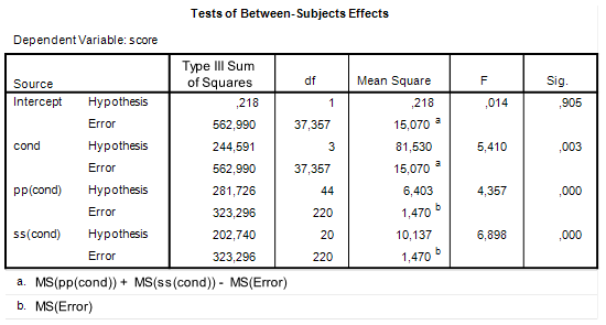
Let us get back to some of the SPSS output we considered in the previous post to get the ingredients we need for sample size planning. First, the ANOVA table.
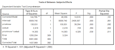 |
| Table 1. ANOVA source table |
We are interested in estimating and optimizing the precision of an interaction contrast estimate. The first things we need are an expression of the error variance needed to calculate the standard error of the estimate and the degrees of freedom that were used in estimating the error variance. In general, the error variance needed is the same error variance you would use in performing an F-test for the specific effect, in this case the interaction effect.
Thus, we note the error variance used to test the interaction effect, i.e. mean square error, and the degrees of freedom. The value of mean square error is 3.324, and the degrees of freedom are 389. Note that this value is the total sample sizes minus the number of conditions (393 – 4 = 389), or, equivalently, the total sample sizes minus the degrees of freedom of the intercept, the main effects, and the interaction (393 – (1 + 1 + 1 + 1) = 389). I will call these degrees of freedom the error degrees of freedom, dfe.
MOE can be obtained by multiplying a critical t-value with the same degrees of freedom as the error degrees of freedom with the standard error of the estimate.
The standard error of the contrast estimate is
![\[\hat{\sigma_\psi}= \sqrt{\sum{c_i^2MS_e/n_i}},\]](https://small-s.science/wp-content/ql-cache/quicklatex.com-e711016f1b800409ee4d1632159091d7_l3.png "Rendered by QuickLaTeX.com")
where  is the contrast weight for the i-th condition mean, and
  the number of observations (in our example participants) in treatment condition i. Note that
  is the variance of treatment mean i, the square root of which gives the familiar standard error of the mean.
The contrast weights we used to estimate the 2 x 2 interaction were {-1, 1, 1, -1}. So, the expression for MOE becomes
![\[MOE = t_{.975}(df_e)\sqrt{\sum{c_i^2MS_e/n_i}}=t_{.975}(df_e)\sqrt{4MS_e/n_i} = 2t_{.975}(df_e)\sqrt{MS_e/n_i}.\]](https://small-s.science/wp-content/ql-cache/quicklatex.com-c566353662177824c69974b4d59785d4_l3.png "Rendered by QuickLaTeX.com")
Thus, suppose we have the independent 2×2 factorial design,  , and the true value of Mean Square Error is 3.324, then MOE for the contrast estimate equals
![\[MOE = 2*t_{.975}(396)*\sqrt{3.324/100} = 0.7071\]](https://small-s.science/wp-content/ql-cache/quicklatex.com-98e408fbb1899034420a41dc86f58115_l3.png "Rendered by QuickLaTeX.com")
.
Note that this is the value of MOE we obtain on average in repeated replications with new samples, if we use sample sizes of 100 (total number of participants is 400) and if the true value of the error variance is 3.324. The value is close to the value we obtained in the previous post (MOE = 0.72) because the sample sizes were very close to 100 per group.
Now, we found the original confidence interval too wide, and we have just seen how 100 participants per group does not really help. MOE is only slightly smaller than our originally obtained MOE. We need to set a target MOE and then figure out how many participants we need to get that target MOE.
Intermezzo: Rules of thumb for target MOE
(Here are some updated rules of thumb: https://the-small-s-scientist.blogspot.com/2018/11/contrast-tutorial.html)
In the absence of theoretical or practical considerations about the precision we want, we may want to use rules of thumb. My (very first proposal for) rules of thumb are based on the default interpretations of Cohen’s d. Considering the absolute values of d ≤ .10 to be negligible d = .20 small, d = .50 medium and d = .80 large. (I really do not like rules-of-thumb, because using them is a sign that you are not thinking).
Now, suppose that we interpret the confidence interval as a range of plausible values for the true value of the effect size. It is not at all clear to me what such a supposition entails, but let’s simply take it for granted right now (please don’t). Then, I think it is reasonable to say that being able to distinguish between small and negligible effects sizes is relatively precise. Thus a MOE of .05 (pooled) standard deviations can be considered precise because (on average) the 95% CI for the small effect sizes is [.15, .25], assuming we know the value of the standard deviation, so negligible effects will not be deemed plausible values on average, since effect sizes smaller than .10 are outside the interval.
By essentially the same reasoning. if we cannot distinguish between large and negligible effects, we are not estimating things very precisely. Therefore, a MOE of .80 standard deviations can be considered to be not very precise. On average, the CI for an existing large effect, will be [0, 1.60], so it includes both negligible and very large effects as plausible values.
For medium (does it make sense to speak of medium precision?) precision I would like to suggest .20-.25 standard deviations. On average, with this value for MOE, if there is a medium effect, small effects and large effects are relatively implausible. In the case of small effects, medium precision entails that on average both effects in the opposite direction and medium effects are among the plausible values.
Of course, I am interpreting the d-values as strict boundaries, but the scale is not categorical, but continuous. So instead of small, large effect sizes, it’s better to speak of smallish and largish effect sizes. And as soon as I find a variant for medium effects sizes I will also include that term in the list.
Note: sample size planning may indicate that precision of MOE = .20-.25 standard deviations is unattainable. In that case, we will simply have to accept that our precision does not lead to confident conclusions about the population effect size. (Once I showed one of my colleagues my precision app, during which he said: “that amount of precision requires a very large sample. I do not like your ideas about sample size planning”).
(By the way, I am also considering rules-of-thumb for target MOE that include assurance. Something like: high precision is when repeated experiments have a high probability of distinguishing small and negligible effects; in that case the average MOE will be smaller than .05).
Planning for precision
Let’s plan for a precision of 0.25 standard deviation. In our case, that standard deviation is the pooled standard deviation: the square root of Mean Square Error. The (estimated) value of Mean Square Error is 3.324 (see Table 1), so our value for the standard deviation is 1.8232. Our target MOE is, therefore, 0.4558.
Let’s make things very clear. Here we are planning for a target MOE based on an estimate of the pooled standard deviation (and on assumptions about the population distribution). In order for our planning to be of practical value, we need some reassurance that that estimate is trustworthy. One way of doing that is to consider the CI for the standard deviation. I will not discuss that topic, and simply give you a CI: [2.90, 3.86].
Take a look at the expression for MOE.
![\[MOE = 2*t_{.975}(df_e)\sqrt{(MS_w / n_i)},\]](https://small-s.science/wp-content/ql-cache/quicklatex.com-1984a751953fc6b0698d72e7bf2c550b_l3.png "Rendered by QuickLaTeX.com")
where  , since we are considering the 2×2 design.
Since our target MOE equals .4588, our goal becomes to solve the following equation for
, since we want the sample size:
However, because
determines both the standard error and the degrees of freedom (and thereby the critical value of t), the equation may be a little hard to solve. So, I will create a function in R that enables me to quite easily get the required sample size. (It is relatively easy to create a more general function (see the Precision App), but here I will give an example tailored to the specific situation at hand).
First we create a function to calculate MOE:
MOE = function(n) {
  MOE = 2*qt(.975, 4*(n - 1))*sqrt(3.324/n)
}
Next, we will define a loss function and use R’s built-in optimize function to determine the sample size. Note that the loss-function calculates the squared difference between MOE based on a sample size n and our target MOE. The optimize function minimizes that squared difference in terms of sample size n (starting with n = 100 and stopping at n = 1000).
loss <- function(n) {
  (MOE(n) - 0.4558)^2
}

optimize(loss, c(100, 1000))
## $minimum
## [1] 246.4563
##
## $objective
## [1] 8.591375e-18
Thus, according to the optimize function we need 247 participants (per group; total N = 988), to get an expected MOE equal to our target MOE. The expected MOE equals 0.4553, which you can confirm by using the MOE function we made above.
Planning with assurance
Although expected MOE is close to our target MOE, there is a probability 50% that the obtained MOE will be larger than our target MOE. In other words, repeated sampling will lead to obtained MOEs larger than what we want. That is to say, we have 50% assurance that our obtained MOE will be at least as small as our target MOE.
Planning with assurance means that we aim for a certain specified assurance that our obtained MOE will not exceed our target MOE. For instance, we may want to have 80% assurance that our obtained MOE will not exceed our target MOE.
![\[MOE_{\gamma} = 2*t_{.975}(df)*\sqrt{MS_w/n_i*\chi^2_{\gamma}(df)/df},\]](https://small-s.science/wp-content/ql-cache/quicklatex.com-f5945fe8ef0dad8f2bf28d70a7553fae_l3.png "Rendered by QuickLaTeX.com")
where  is the assurance expressed in a probability between 0 and 1.
Let’s do it in R. Again, the function that calculates assurance MOE is tailored for the specific situation, but it is relatively easy to formulate these functions in a generally applicable way,
MOE.gamma = function(n) {
  df = 4*(n-1)
  MOE = 2*qt(.975, df)*sqrt(3.324/n*qchisq(.80, df)/df)
}
loss <- function(n) {
  (MOE.gamma(n) - 0.4558)^2
}

optimize(loss, c(100, 1000))
## $minimum
## [1] 255.576
##
## $objective
## [1] 2.900716e-18
Thus, according to the results, we need 256 persons per group (N = 1024 in total) to have a 80% probability of obtaining a MOE not larger than our target MOE. In that case, our expected MOE will be 0.4472.


![\[\sigma_{\hat{\psi}} = \sqrt{\sum{w_i}\sigma^2_e/n}\]](https://small-s.science/wp-content/ql-cache/quicklatex.com-14bc511e9204319eaaccbcfd696c36c3_l3.png "Rendered by QuickLaTeX.com")
 ) .
) .![\[\sigma^2_e = \sigma^2_{within}(1 - \rho)\]](https://small-s.science/wp-content/ql-cache/quicklatex.com-beec527cea79344408614018693eb04e_l3.png "Rendered by QuickLaTeX.com")

 . Now, suppose that due to some freak accident of nature there are no differences in the mean scores (averaged of stimuli) of each participant. In that case,
  . This means that under these circumstances the expected mean square associated with participants is simply an estimate of the error variance with
  degrees of freedom, because
  , if
, if  degrees of freedom. The logic of the F-test is that under the null-hypothesis, in our case that
  . If we now suppose that there is no difference between the treatment means, that is
  , MSTreatment does not estimate
  , but
, but  . Note that no other source of variance has an expected mean square that is equal to the latter figure. That is, in contrast to our test of the Participant factor, where under the null-hypotheses two Mean Squares estimate the error variance, i.e. MSParticipant and MSError, no mean square is available to form an F-ratio to test the Treatment effect.
![[m\sigma^2_p + \sigma^2_e] + [m\sigma^2_s + \sigma^2_e] - [\sigma^2_e] = m\sigma^2_p + n\sigma^2_s + \sigma^2_e](https://small-s.science/wp-content/ql-cache/quicklatex.com-9cd6bb15506816413e74641fee23cf13_l3.png "Rendered by QuickLaTeX.com") . It is exactly this linear combination of mean squares that is used in the F-ratio to obtain an error term against which to test the Treatment effect in Figure 1:
. It is exactly this linear combination of mean squares that is used in the F-ratio to obtain an error term against which to test the Treatment effect in Figure 1:  . We will also use this figure to obtain the variance (and standard error) of our contrast estimate.
![\[df=\frac{(MSp+MSs-MSe)^{2}}{\frac{MSp^{2}}{df_{p}}+\frac{MSs^{2}}{df_{s}}+\frac{MSe^{2}}{df_{e}}}.\]](https://small-s.science/wp-content/ql-cache/quicklatex.com-13f753be88a6e13890953c2465e22a05_l3.png "Rendered by QuickLaTeX.com")
 can be obtained as follows.
![\[\hat{\sigma}_{\hat{\psi}}=\sqrt{\sum c_{i}^{2}\hat{\sigma}_{\bar{X},Rel}^{2}},\]](https://small-s.science/wp-content/ql-cache/quicklatex.com-489e315828278a9811848f3ce71bf10f_l3.png "Rendered by QuickLaTeX.com")
 to refer to the relative error variance of the treatment mean (which in this design is equal to the absolute error variance, but that’s another story), and
  . Thus, using the results in Figure 1.
![\[\hat{\sigma}_{\bar{X},Rel}^{2}=\frac{MS_{p}+MS_{s}-MS_{e}}{nm}=\frac{15.07}{72}=0.2093.\]](https://small-s.science/wp-content/ql-cache/quicklatex.com-0d81fe2ec65ea2c26c84682713e499bf_l3.png "Rendered by QuickLaTeX.com")
 . Let’s use the results in Figure 1 to calculate what MOE is for this particular contrast.
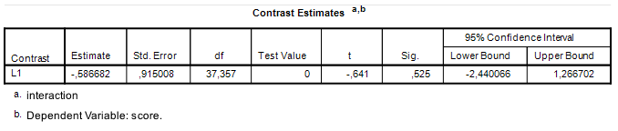
 , with 220 degrees of freedom and not
  , with 37.357 (see Figure 1). The consequence of this is, of course, that the 95% CI is much narrower than it should be.
 , the critical value of t is the .975 quantile of the central t distribution with
  , which equals
  . The value of MOE is therefore
  . With a contrast estimate of
  , the 95% CI equals
 ![-0.587 \pm 0.5633 = [-1.1503, -0.0237]](https://small-s.science/wp-content/ql-cache/quicklatex.com-ea5612615f1baf096374644a223d775f_l3.png "Rendered by QuickLaTeX.com") . In comparison, using the correct value of MOE gives us
. In comparison, using the correct value of MOE gives us ![[−2.4404, 1.2664]](https://small-s.science/wp-content/ql-cache/quicklatex.com-ef97651e8790dc304790e8a8724ebed7_l3.png "Rendered by QuickLaTeX.com") .
.
 , approximate 95% CI
 ![[-1.40, 0.73]](https://small-s.science/wp-content/ql-cache/quicklatex.com-867264624a612f401b2c1cea536372a9_l3.png "Rendered by QuickLaTeX.com") , which according to the rules of thumb is a medium negative effect, but consistent with anytihing from a huge negative effect to a large positive effect in the population, as the approximate CI shows. (I have divided the point estimate and the confidence interval in Figure 2 by 1.74, to obtain Cohen’s d and an approximate confidence interval). Clearly, then, our precision can be optimized.
, which according to the rules of thumb is a medium negative effect, but consistent with anytihing from a huge negative effect to a large positive effect in the population, as the approximate CI shows. (I have divided the point estimate and the confidence interval in Figure 2 by 1.74, to obtain Cohen’s d and an approximate confidence interval). Clearly, then, our precision can be optimized. , the stimulus variance
  , and the error variance
  . Rearranging and using 1.47 as an estimate for
  . Likewise, the estimate for
  . Thus, our estimates are
  ,
,  , and
, and  .
.
 , for assurance the value .80 and the values
  , and
, and  for, respectively, Residual variance, Participant intercept variance and Stimulus intercept variance. Fill in the value 0 for all the other variances. See Figure 5.

 , to refer to the residual variance in the BwC-design, we can say
  . Normally, the precision app sums these two components to get a value for the residual variance in the BwC-design, and you will obviously get the same result if you specify the residual variance as the sum and the participant-by-stimulus variance as 0. Likewise,
  , and
, and  , where
  and
and  are the variances associated with the interaction of treatment and participant and treatment and stimulus, respectively.
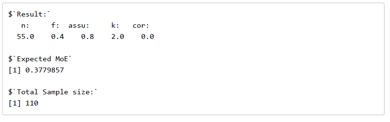
 , and there is 80% assurance that MOE will not exceed
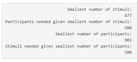
  . Note, again, that the assurance MOE is somewhat larger than target MOE, because a sample of 804 participants requires a sample of more than 500 stimuli to get the target MOE with 80% assurance and 500 stimuli is the maximum number of stimuli the app considers when minimizing the number of participants.

 ,
,  ,
,  ,
,  ,
,  , and
, and  . The Satterthwaite degrees of freedom are
  . The standard error of the contrast equals
  . The critical value for t equals
  . Expected MOE is, therefore,
  (the tiny difference with the results from the app is due to rounding errors).
 -distribution. That is, we assume with assurance
  , that the
  . Now, the degrees of freedom are
  , the assurance
  , and the .80 quantile of
  . Since the relative error variance equals
  , the .80 quantile of the error variance equals
  . And this means that assurance MOE equals
  . Again, the difference with the results from the Precision App are due to rounding error.
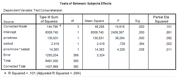
![\[0.4558 = 2*t_{.975}(4(n_i - 1)\sqrt{(MS_w / n_i)},\]](https://small-s.science/wp-content/ql-cache/quicklatex.com-9a775e47b691309421ea2f9d94c016c2_l3.png "Rendered by QuickLaTeX.com")