Planning for Precise Contrast Estimates: Introduction and Tutorial (Preprint)

I just finished a preprint of an introduction and tutorial to sample size planning for precision of contrast estimates. The tutorial focuses on single factor between and within subjects designs, and mixed factorial designs with one within and one between factor. The tutorial contains R-code for sample size planning in these designs.

The preprint is availabe on researchgate: Click (but I am just as happy to send it to you if you like; just let me know).

Planning with assurance, with assurance

Planning for precision requires that we choose a target Margin of Error (MoE; see this post for an introduction to the basic concepts) and a value for assurance, the probability that MoE will not exceed our target MoE.  What your exact target MoE will be depends on your research goals, of course.

Cumming and Calin-Jageman (2017, p. 277) propose a strategy for determining target MoE. You can use this strategy if your research goal is to provide strong evidence that the effect size is non-zero. The strategy is to divide the expected value of the difference by two, and to use that result as your target MoE.

Let’s restrict our attention to the comparison of two means. If the expected difference between the two means is Cohens’s d = .80, the proposed strategy is to set your target MoE at f = .40, which means that your target MoE is set at .40 standard deviations. If you plan for this value of target MoE with 80% assurance, the recommended sample size is n = 55 participants per group. These results are guaranteed to be true, if it is known for a fact that Cohen’s d is .80 and all statistical assumptions apply.

But it is generally not known for a fact that Cohen’s d has a particular value and so we need to answer a non-trivial question: what effect size can we reasonably expect? And, how can we have assurance that the MoE will not exceed half the unknown true effect size? One of the many options we have for answering this question is to conduct a pilot study, estimate the plausible values of the effect size and use these values for sample size planning.  I will describe a strategy that basically mirrors the sample size planning for power approach described by Anderson, Kelley, and Maxwell (2017).

The procedure is as follows. In order to plan with approximately 80% assurance, estimate on the basis of your pilot the 80% confidence interval for the population effect size and use half the value of the lower limit for sample size planning with 90% assurance. This will give you 81% assurance that assurance MoE is no larger than half the unknown true effect size.

The logic of planning with assurance, with assurance

There are two “problems” we need to consider when estimating the true effect size. The first problem is that there is at least 50% probability of obtaining an overestimate of the true effect size. If that happens, and we take the point estimate of the effect size as input for sample size planning, what we “believe” to be a sample size sufficient for 80% assurance will be a sample size that has less than 80% assurance at least 50% of the times. So, using the point estimate gives assurance MoE for the unknown effect size with less than 50% assurance.

To make it more concrete: suppose the true effect equals .80, and we use n = 25 participants in both groups of the pilot study, the probability is  approximately 50% that the point estimate is above .80. This implies, of course, that we will plan for a value of f > .40, approximately 50% of the times, and so the sample we get will only give us 80% assurance 50% of the times.

The second problem is that the small sample sizes we normally use for pilot studies may give highly imprecise estimates. For instance, with n = 25 participants per group, the expected MoE is f = 0.5687. So, even if we accept 50% assurance, it is highly likely that the point estimate is rather imprecise.

Since we are considering a pilot study,  one of the obvious solutions, increasing the sample size so that expected MoE is likely to be small, is not really an option. But what we can do is to use an estimate that is unlikely to be an overestimate of the true effect size. In particular, we can use as our estimate the lower limit of a confidence interval for the effect size.

Let me explain, by considering the 80% CI  of the effect size estimate. From basic theory it follows that the “true” value of the effect size will be smaller than the lower limit of the 80% confidence interval with probability  equal to 10%. That is, if we calculate a huge number of 80% confidence intervals, each time on the basis of new random samples from the population, the true value of the effect size will be below the lower limit in 10% of the cases. This also means that the lower limit of the interval has 90% probability to not overestimate the true effect size.

This means that  if we take the lower limit of the 80% CI of the pilot estimate as input for our sample size calculations, and if we plan with assurance of .90, we will have 90%*90% = 81% assurance that using the sample size we get from our calculations will have  MoE  no larger than half the true effect size. (Note that for 80% CI’s with negative limits you should choose the upper limit).

Sample Size planning based on a pilot study

Student of mine recently did a pilot study.  This was a pilot for an experiment investigating the size of the effect of fluency of delivery of a spoken message in a video on Comprehensibility, Persuasiveness and viewers’ Appreciation of the video. The pilot study used two groups of size n = 10, one group watched the fluent video (without ‘eh’) and the other group watched the disfluent video where the speaker used ‘eh’ a lot. The dependent variables were measured on 7-point scales.

Let’s look at the results for the Appreciation variable. The (biased) estimate of Cohen’s d (based on the pooled standard deviation) equals 1.09, 80% CI [0.46, 1.69] (I’ve calculated this using the ci.smd function from the MBESS-package. According to the rules-of-thumb for interpreting Cohen’s d, this can be considered a large effect. (For communication effect studies it can be considered an insanely large effect). However, the CI shows the large imprecision of the result, which is of course what we can expect with sample sizes of n = 10. (Average MoE equals f = 0.95, and according to my rules-of-thumb that is well below what I consider to be borderline precise).

If we use the lower limit of the interval (d = 0.46),  sample size planning with 90% assurance for half that effect (f = 0.23) gives us a sample size equal to n = 162. (Technical note: I planned  for the half-width of the standardized CI of the unstandardized effect size, not for the CI of the standardized effect size; I used my Shiny App for planning assuming an independent groups design with two groups).  As explained, since we used the lower limit of the 80% CI of the pilot and used 90% assurance in planning the sample size, the assurance that MoE will not exceed half the unknown true effect size equals 81%.

Contrast Analysis with R for factorial designs: A Tutorial

In this post, I want to show how to do contrast analysis with R for factorial designs. We focus on a 2-way between subjects design. A tutorial for factorial within-subjects designs can be found here: https://small-s.science/2019/01/contrast-analysis-with-r-repeated-measures/ . A tutorial for mixed designs (combining within and between subjects factors can be found here: https://small-s.science/2019/04/contrast-analysis-with-r-mixed-design/.

I want to show how we can use R for contrast analysis of an interaction effect in a 2 x 4 between subjects design. The analysis onsiders the effect of students’ seating distance from the teacher and the educational performance of the students: the closer to the teacher the student is seated, the higher the performance. A “theory “explaining the effect is that the effect is mainly caused by the teacher having decreased levels of eye contact with the students sitting farther to the back in the lecture hall.

To test that theory, a experiment was conducted with N = 72 participants attending a lecture. The lecture was given to two independent groups of 36 participants. The first group attended the lecture while the teacher was wearing dark sunglasses, the second group attented the lecture while the teacher was not wearing sunglasses. All participants were randomly assigned to 1 of 4 possible rows, with row 1 being closest to the teacher and row 4 the furthest from the teacher The dependent variable was the score on a 10-item questionnaire about the contents of the lecture. So, we have a 2 by 4 factorial design, with n = 9 participants in each combination of the factor levels. 

Here we focus on obtaining an interaction contrast: we will estimate the extent to which the difference between the mean retention score of the participants on the first row and those on the other rows differs between the conditions with and without sunglasses. 

The interaction contrast with SPSS

I’ve downloaded a dataset from the supplementary materials accompanying Haans (2018) from http://pareonline.net/sup/v23n9.zip (Between2by4data.sav) and I ran the following syntax in SPSS:

UNIANOVA retention BY sunglasses location
 /LMATRIX = "Interaction contrast" 
  sunglasses*location 1 -1/3 -1/3 -1/3 -1 1/3 1/3 1/3 intercept 0
   /DESIGN= sunglasses*location.

Table 1 is the relevant part of the output.

SPSS Interaction Contrast
Table 1. Spss ouput for the interaction contrast

So, the estimate of the interaction contrasts equals 1.00, 95% CI [-0.332, 2.332]. (See this post for optimizing the sample size to get a more precise estimate than this).

Contrast analysis with R for factorial designs

Let’s see how we can get the same results with R.

library(MASS)
library(foreign)

theData <- read.spss("./Between2by4data.sav")
theData <- as.data.frame(theData)

attach(theData)

# setting contrasts 
contrasts(sunglasses) <- ginv(rbind(c(1, -1)))
contrasts(location)  <- ginv(rbind(c(1, -1/3, -1/3, -1/3),
                                   c(0, 1, -1/2, -1/2), c(0, 0, 1, -1)))

# fitting model

myMod <- lm(retention ~ sunglasses*location)

The code above achieves the following. First the relevant packages are loaded. The MASS package provides the function ginv, which we need to specify custom contrasts and the Foreign package contains the function read.spss, which enables R to read SPSS .sav datafiles.

Getting custom contrast estimates involves calculating the generalized inverse of the contrast matrices for the two factors. Each contrast is specified on the rows of these contrast matrices. For instance, the contrast matrix for the factor location, which has 4 levels, consists of 3 rows and 4 columns. In the above code, the matrix is specified with the function rbind, which basically says that the three contrast weight vectors c(1, -1/3, -1/3, -1/3), c(0, 1, -1/2, -1/2), c(0, 0, 1, -1) form the three rows of the contrast matrix that we use as an argument of the ginv function. (Note that the set of contrasts consists of orthogonal Helmert contrasts).

The last call is our call to the lm-function which estimates the contrasts. Let’s have a look at these estimates.

summary(myMod)
## 
## Call:
## lm(formula = retention ~ sunglasses * location)
## 
## Residuals:
##    Min     1Q Median     3Q    Max 
##     -2     -1      0      1      2 
## 
## Coefficients:
##                       Estimate Std. Error t value Pr(>|t|)    
## (Intercept)             5.3750     0.1443  37.239  < 2e-16 ***
## sunglasses1             1.2500     0.2887   4.330 5.35e-05 ***
## location1               2.1667     0.3333   6.500 1.39e-08 ***
## location2               1.0000     0.3536   2.828  0.00624 ** 
## location3               2.0000     0.4082   4.899 6.88e-06 ***
## sunglasses1:location1   1.0000     0.6667   1.500  0.13853    
## sunglasses1:location2   3.0000     0.7071   4.243 7.26e-05 ***
## sunglasses1:location3   2.0000     0.8165   2.449  0.01705 *  
## ---
## Signif. codes:  0 '***' 0.001 '**' 0.01 '*' 0.05 '.' 0.1 ' ' 1
## 
## Residual standard error: 1.225 on 64 degrees of freedom
## Multiple R-squared:  0.6508, Adjusted R-squared:  0.6126 
## F-statistic: 17.04 on 7 and 64 DF,  p-value: 1.7e-12

For the present purposes, we will consider the estimate of the first interaction contrast, which estimates the difference between the means of the first and  the other rows between the with and without sunglasses conditions. So, we will have to look at the sunglasses1:location1 row of the output.

Unsurprisingly, the estimate of the contrast and its standard error are the same as in the SPSS ouput in Table 1. The estimate equals 1.00 and the standard error equals 0.6667.

Note that the residual degrees of freedom equal 64. This is equal to the product of the number of levels of each factor, 2 and 4, and the number of participants (9) per combination of the levels minus 1: df =  2*4*(9 – 1) = 64. We will use these degrees of freedom to obtain a confidence interval of the estimate.

We will calculate the confidence interval by first extracting the contrast estimate and the standard error,  after which we multiply the standard error by the critical value of t with df = 64 and add the result to and substract it from the contrast estimate:

estimate = myMod$coefficients["sunglasses1:location1"]

se = sqrt(diag(vcov(myMod)))["sunglasses1:location1"]

df = 2*4*(9 - 1)

# confidence interval

estimate + c(-qt(.975, df), qt(.975, df))*se
## [1] -0.3318198  2.3318198


Clearly, we have replicated all the estimation results presented in Table 1.

Reference
Haans, Antal (2018). Contrast Analysis: A Tutorial. Practical AssessmentResearch& Education, 23(9). Available online: http://pareonline.net/getvn.asp?v=23&n=9

Planning for precise contrast estimates in between subjects designs

Here I would like to explain the procedure for sample size planning for one-way and two-way (factorial) between subjects designs. We will consider examples based on and described in Haans (2018).

The first example: one-way design

The first example considers the effect of seating location  of students on their educational performance. Seating location is defined as distance from the teacher and operationalized in terms of the row the student is seated in, with first row being the closest to the teacher and the fourth row being the furthest away. 20 Students are randomly assigned to one of the four possible rows, so N = 20, n = 5. The dependent variable is the course grade of the student. (Note: the data and study are hypothetical).

As Haans (2018) explains, one psychological theory explaining the effect of seating position on educational performance is based on social influence. This theory posits that due to the social influence of the teacher, the students that are seated closest to the teacher find themselves in a state of undivided attention. This undivided attention causes their educational performance to be better than the students who are seated further away.

In operational terms, then, we may expect that first row students will have a better average grade than students seated on the other rows. So, the quantitative research question we are interested in is:

“How much do the average grades differ between students seated first row and the students seated on other rows?”

We can estimate this quantity with a Helmert Contrast, where we assign a contrast weight of 1 to mean of the first row grades and weights -1/3 to the means of the grades in the other rows.

Haans (2018) gives us the following results. The contrast estimate equals 2.00 , 95% CI [0.27, 3.73]. In order to interpret this more easily, we divide this estimate by the square root Mean Square Error, to obtain the standardized estimate and standardized confidence interval (not to be confused with the confidence interval of the standardized estimate, but that’s a different story. The result is: 1.26, 95% CI [0.17, 2.36].

To answer the research question, the estimated difference equals 1.26 standard deviations, which according to rule-of-thumbs frequently used in psychology is a large difference. The CI shows the enormous amount of uncertainty of this estimate: population values between 0.17 (small) and 2.36 (very large) are also consistent with the observed data and our statistical assumptions. So, it seems safe to conclude that it looks like there is a positive effect of seating position, but the wide range of the CI makes it clear that the data do not tell us enough about the size of the effect, the precision is simply too low.

The precision is f = 1.09, which according to my rules-of-thumb is very imprecise (I consider f = 0.65, to be barely tolerable).

So, let’s plan for a replication study with a reasonably precise estimate of  f = 0.40, with 80% assurance. (Note: for some advice on setting target Moe: Planning with assurance, with assurance. ) I’ve used the app: https://gmulder.shinyapps.io/PlanningFactorialContrasts/ with the default values for a single factor between subjects design with 4 conditions.  According to the app, we need n = 36 participants per condition (making a total of  N = 144).

(For more detailed information considering sample size planning for contrast analysis see: http://small-s.science/?p=10 and for some guidelines for setting target MoE: http://small-s.science/?p=14)

The second example: factorial design

Our second example is also taken from Haans (2018). It considered the same phenomenon, the effect of students’ seating distance from the teacher and the educational performance of the students.

A second theory explaining the effect is that the effect is mainly caused by the teacher having decreased levels of eye contact with the students sitting farther to the back in the lecture hall.

To test that theory, a experiment was conducted with N = 72 participants attending a lecture. The lecture was given to two independent groups of 36 pariticpant. The first group attended the lecture while the teacher was wearing dark sunglasses, the second group attented the lecture while the teacher was not wearing sunglasses,. Again, all participants were randomly assigned to 1 of 4 possible rows. The dependent variable was the score on a 10-item questionnaire about the contents of the lecture.

Now, if the eyecontact of the teachter is the causal variable, we may expect that in this experimental setup the difference between the average score of the persons seated on the first row and the averages of the other rows will be smaller for the condition where the teacher wears sunglasses than for the condition in which the teacher does not wear these glasses, as wearing sunglasses prevents eye-contact between the teacher and the students. Our quantitative question is therefore:

“How much does the contrast between the first row and the others rows differ between the conditions with and without sunglasses?”

In other words, we are interested in the size of the interaction effect.

I’ve downloaded the dataset from http://pareonline.net/sup/v23n9.zip (between2by4data.sav) and specified the following syntax in SPSS:

UNIANOVA retention BY sunglasses location
 /LMATRIX = “Interaction contrast” sunglasses*location 1 -1/3 -1/3 – 1/3 -1 1/3 1/3 1/3 intercept 0
  /DESIGN= sunglasses*location.

The result of the analysis is that the contrast estimate equals 1.0, 95% CI [-0.33, 2.33]. If we standardize this with the within condition variance (the condition being the combination of the levels of the two factors), we get 0.82, 95% CI [-0.27, 1.90].

So, it appears that the difference between the means of the first row and that of the other rows is on average 1.0 points larger in the condition without sunglasses than in the condition with sunglasses. This corresponds to a large difference (dwith = .82). However, the CI also contains negative population difference (albeit that they are smallish), so even though the results are promising for the theory (eyecontact), these negative effects will not persuade a critical reviewer of the study. Indeed, these negative effects contradict the substantive hypothesis.

Again, the confidence interval is so wide, that effects ranging from small negative effects to huge positive effects are considered plausible. Since the results are promising for the theory, a replication study with more precision may be needed to persuade the critics. Let’s plan for a precision of f = .25 with 95% assurance.

I’ve used the app: https://gmulder.shinyapps.io/PlanningFactorialContrasts/ specifying that we have a factorial design with a = 2 levels and b = 4 levels. The result is that for the interaction contrast  with f = .25 and assurance = .95, we need 175 participants per combination of the two factors. This means, that a total of N = 1400 must be recruited.

I’ve taken this from the following output.

Planning for precision of a contrast estimate
Figure 1: Output of sample size planning 

I’ve looked at the  “Contrast Summary Tab” to check that interaction A1B1 is the correct one (see Figure 2).

Interaction contrast weights
Figure 2. Summary of contrast weights.

What’s important in the above figure is that the set of weights for A1B1 matches the set of weights used to get the contrast estimate in SPSS (In the LMATRIX-subcommand), so that’s how we know that A1B1 is the contrast we want.  (Note: if you switch the number of levels in the app, that is, use 4 levels for A and 2 for B, the interaction weights will match perfectly).

Reference
Haans, Antal (2018). Contrast Analysis: A Tutorial. Practical Assessment, Research, & Education, 23(9). Available online: http://pareonline.net/getvn.asp?v=23&n=9

Planning for precise contrasts in two-way factorial designs: a Tutorial

I’ve created a first version of Shiny App for sample size planning for precise contrast estimates in one and two-way designs. So, if you want to plan for interaction contrasts for two-way designs, take a look here: https://gmulder.shinyapps.io/PlanningFactorialContrasts/

Important: this is a first version that contains no error checking (but you know what you’re doing, so that’s not a problem). Also, I have not tested the results of the app with simulation studies. As soon as I have done that, I will share the code of the app.

Update: The values for the factorial two-way within subjects designs are checked with simulation studies (for f = .40, assurance = .80, and correlation rho = .50).

Note: if you have a single factor design, you may also consider looking here: http://small-s.science/?p=19

Note: if you have a two-groups independent design, go here for an introduction to sample size planning and its relation to the power of the t-test: http://small-s.science/?p=25

See for more detailed information about sample size planning for single factor and factorial designs (between, within, and mixed): http://small-s.science/?p=10 and for guidelines for setting target MoE: http://small-s.science/?p=14)

How does the app work?

1. Specifying Target MoE and Assurance 

Target MoE should be specified in a number of standard deviations (usually a fraction; for details see Cumming, 2012; Cumming & Calin-Jageman, 2017). The symbol f will be used to refer to this standardized MoE. Target MoE (f) must be larger than zero (f will be automatically set to .05 if you accidentally fill in the value 0). 
I suggest using the following guidelines for target MoE (f): 
Description f
Extremely Precise .05
Very Precise .10
Precise .25
Reasonably Precise .40
Borderline Precise .65
You should only use these guidelines if you lack the information you need for specifying a reasonable value for Target MoE.

Assurance is the probability that (to be) obtained MoE will be no larger than Target MoE. I suggest setting Assurance minimally at .80.

Assumptions of the App

The app uses the within condition standard deviation as the standardizer for MoE. For the factorial designs this is the variance within each combination of the factor levels. The app assumes equal variances and, for the mixed and within subject designs equal covariances as well.

2. Specifying number of factors, design, correlation and levels of each factor 

You can plan for designs with one factor (between and within designs) and two factors (between, within, and mixed designs).  
If you have a mixed design, the first factor (Factor A) is considered to be the between subjects factor and the second factor (Factor B) the within subjects factor. 
The app also requires a value for the cross-condition correlation in the within or mixed designs. 

3. Specifying contrasts 

Main comparisons 

The default contrasts for main comparisons are Helmert contrasts, but you can specify any contrast you like. Use commas to separate the contrast weights and use semi-colons to separate the weights of different contrasts. For example, the “1, -1/2, -1/2; 0, 1, -1” indicates two contrasts, the first contrast has weights {1, -1/2, -1/2}, the second contrast has weights {0, 1, -1}. 
It is recommended that the absolute values of the contrast weights of each contrast sum to 2.0 (except for interaction contrasts, where the absolute values should sum to 4.0). 
You will only have to specify contrasts for the marginal means of each factor. The app calculates appropriate values for the contrast weights of each cell in the design based on the weights for the marginal means. For example, in a 2×2 design the weights for the marginal means for each factor may be {1, -1]. The app translates this to {0.5, 0.5, -0.5, -0.5}, to account for the fact that the contrast etimates involves the combination of each of the 2×2 cell means.

Interaction contrasts 

The app calculates the interaction contrasts on the basis of the contrasts specified for the main comparisons. So, if you want to plan for your favorite interaction, simply type in the weights for the two main comparisons involved. Suppose you have a 2×2 design, for example, and you want to plan for an interaction contrasts with weigths {1, -1, -1, 1}, type in “1, -1” for factor A and “1, -1” for factor B. 
As another example, suppose factor A has two levels and factor B has three, and you want to estimate the extent to which the difference between the first level of B and the means of the other two levels differes between the levels of A. You type in “1, -1” for factor A, and  “1, -1/2, -1/2” for factor B, and the app will calculate the interaction contrast with weights {1, -1/2, -1/2, -1, 1/2, 1/2}. 
After planning the results: you can check whether the contrasts are what you intended by looking at the “Contrast Summary” output-tab. 

4. Output 

The output contains sample sizes  per  treatment (combination) and total samples required for target MoE and assurance. You will get samples sizes per contrast. 
On the “Contrasts Summary” tab the app shows information about the contrast weights. 

Planning for Precise Contrasts: Tutorial for single factor designs

This is a tutorial for  a planning for precision  of contrasts estimates. The application is here: https://gmulder.shinyapps.io/PlanningContrasts/.

NOTE: For a (beta) version of planning for factoral designs: http://small-s.science/?p=18

NOTE: I’ve updated the app with a few corrections, so there is a new version. (The November version has corrected degrees of freedom  for the 3 and 4 condition within design).

If you like to run the app in R, install the shiny and devtool packages and run the following:

library(shiny)
library(devtools)
source_url("https://git.io/fpI1R")
shinyApp(ui = ui, server = server)

Specifying Target MoE and Assurance

Target MoE should be specified in a number of standard deviations (usually a fraction; for details see Cumming, 2012; Cumming & Calin-Jageman, 2017). The symbol f will be used to refer to this standardized MoE. Target MoE (f) must be larger than zero (f will be automatically set to .05 if you accidentally fill in the value 0).
I suggest using the following guidelines for target MoE (f):
Description f
Extremely Precise .05
Very Precise .10
Precise .25
Reasonably Precise .40
Borderline Precise .65
You should only use these guidelines if you lack the information you need for specifying a reasonable value for Target MoE.

Assurance is the probability that (to be) obtained MoE will be no larger than Target MoE. I suggest setting Assurance minimally at .80.

Specifying the Design

The app works with independent and dependent designs for 2, 3, and 4 conditions.  With 2 conditions, the analysis is equivalent to the independent and dependent t-tests, with more than two conditions the analysis is equivalent to one-way independent ANOVA or dependent ANOVA.

Specifying the Cross-Condition correlation

If you choose the dependent design, you also need to specify a value for the cross-condition correlation. This value should be larger than zero. One of the assumptions underlying the app, is that there is only 1 observation per participant (or any other unit of analysis). That is why I like to think of this correlation as (conceptually related to) the reliability of the participant scores (averaged over conditions). From that perspective, a correlation around .60 would be borderline acceptable and around .80 would be considered good enough. So, for worst-case scenarios use a correlation smaller than .60, and for optimistic scenario’s correlations of .80 or larger.

Note: for technical reasons a correlation of 1 will be automatically changed to .99.

For independent designs the correlation should equal 0. (And the above story about reliability does no longer make sense; but we also do not need it).

Specifying Contrasts 

Contrasts must obey the following rules.

  1. The sum of the contrast weights must equal zero;
  2. The sum of the absolute values of the contrast must be equal to two.
If the contrast weights confirm to these rules the resulting estimate is a difference between two or more means expressed on the scale of the variable (see Kline, 2013 for more information on contrasts).
The contrast estimate is simply the sum of the condition means multiplied by the contrast weights. For instance, with four condition means M1, M2, M3, M4, and contrast weights {0.5, 0.5, -0.5, -0.5}, the value of the contrast estimate is the sum 0.5M1 + 0.5M2 + -0.5M3 + -0.5M4 = (.5M1 + .5M2) – (.5M3 + .5M4) = ( M1 + M2) / 2 – (M3 + M4) / 2:  the value of the contrast estimate is the difference between the mean of the first two conditions and the mean of the last two conditions.
With more than 2 conditions, the app let’s you choose between “Custom contrast” and “Helmert Contrasts”.
If you choose “Custom contrast” the app plans for precision of just that contrast. You will get the sample size needed and a figure of the expected results (see below). The default values give you the weights for a pair wise comparison of two of the conditions. You can simply type over these default values.
If you choose “Helmert contrasts” the app will give you an orthogonal set of Helmert contrasts as default values.  You can simply type over these default values to get any contrast you like, but you cannot specify more contrasts than the number of conditions minus one.
If you choose “Helmert contrasts” the app will plan for the sample size of the contrast with the lowest precision. If you use the default values this will be the contrast specifying a pairwise comparison.  For a set of contrasts the pair wise comparison estimate will be the least precise so if you know the sample size needed for a precise pairwise comparison, you know that the precision you will get for the other contrasts will be just as precise  or more precise. The planning results will show the expected value for MoE for all contrasts, but the figure will only display expected results for the least precise contrast estimate.

Examples 

Two groups independent design 
 
I use the default values (see Figures 1 and 2). And click the “Get Sample size ” button.
Figure 1. Values for Target MoE, assurance and design
Figure 2: Standard contrasts for comparison of two conditions

The output is as follows:

The results give you the sample size for each condition (n), and information about target MoE (f), assurance (assu), the number of conditions (k), and the cross-condition correlation (cor; the value is zero, as it should be in the independent design). With n = 55, there is a 80% probability that f will not be larger than .40.

If you use 55 participants per group the expected MoE equals 0.38.

Of course, using 55 participants per group, makes the total sample size equal to 110.

The output also included a plot of the expected results (what you can expect to happen on average). See Figure 3.

Figure 3: Expected results using n = 55 participants per group in the two groups independent design

This output helps you to consider whether the Expected MoE is small enough. Suppose, for instance, that true difference equals .5 standard deviations, i.e. a medium effect. The figure shows that the expected contrast estimate is a medium effect, and the confidence interval shows that on average values ranging from small to large effects [.12, .88] will be included in the interval. If the difference between small, medium and large effects is important, an expected precision of f = .38 may not be enough, although small and large effects are at the limits of the confidence interval.

A four groups dependent design 

Technical Note:
The app assumes that the sum of squares of the Error Variance can be decomposed in (k – 1) equal parts, where k is the number of conditions. I will change this restriction in a future version of the app. For a custom contrast it is assumed that the contrast is part of an orthogonal set.

Suppose your major interest is the comparison between the average of two groups and the average of two other groups. You have a dependent (repeated measures) design in which participants will be exposed to each of the four treatment conditions. Let’s plan for a target MoE of f = 0.25, with 80 % assurance and let’s suppose our cross-condition correlation equals r = .70. I choose a custom contrast with weights {1/2, 1/2, -1/2, -1/2} (see Figure 4).

Figure 4. Input for sample size planning

The output is as follows.

So, we need 26 participants to have 80% assurance that obtained MoE will not be larger than f = 0.25. Expected MoE is equal to .22. According to the guidelines above, this is a precise estimate.

If you choose “Helmert Contrasts” instead, and press the button without changing anything, the output is as follows.

Under Expected Moe you will see for each of the three contrasts c1, c2, and c3, the weights and expected MOE. The 46 participants give an expected MoE smaller than target MoE, for the least precise estimate (c3; the pairwise comparison) the other expected MoE’s are smaller than that. The Expected Results Figure will display the results for the contrasts with the largest expected MoE.


A rule of thumb for setting target MOE

One of the most difficult aspects of sample size planning for precision is the specification of a target Margin of Error (MoE). Here, I would like to introduce a simple rule of thumb, in the hope that it helps you in determining a reasonable target MoE.
Here, the rule of thumb is applied to obtaining an estimate of the difference between two independent group means, where the two populations are normally distributed with equal variances.

Goal 1: Assessing the direction of an effect

Sample size planning starts with formulating a goal for the research. A very common goal is to try to determine the direction of an effect. For the goal of assessing the direction of an effect, it helps if the confidence interval of the difference contains only positive or negative values. That is, you want a confidence interval that exludes the value 0, for if that value is included, you would probably conclude that the estimate is consistent with both positive and negative effects. Thus, our first goal is to obtain a confidence interval of the mean difference that excludes the value 0.

Now, a confidence interval excludes 0, if obtained MOE is at most equal to the obtained effect size estimate. Suppose that the estimate equals the true effect of say, 0.50, we want MOE to be at most very close to 0.50, otherwise 0 will be included in the interval. But if our estimate underestimates the true effect, say the estimate equals 0.30, we want MOE to be at most very close to 0.30. Likewise, if we overestimate the effect, MOE can be larger than 0.50.

This means that we cannot say, for instance, we expect that the true effect is .50, so let’s plan for a target MOE that with 80% assurance is at most .50, because this target MOE may be too large for underestimates of the true effect, depending on the extent to which the effect is underestimated. So, in specifying target MOE, we should take into account that underestimates of the effect size occur. (Actually, these underestimates occur with a relative frequency of 50% in a huge collection of direct replications). We can say that we do not only want to exclude zero from the interval, but also that we want that to occur in a large proportion of direct replications. This will be our second goal. I will call the probabiity associated with our second goal, the probability of exclusion (PE)

The rule of thumb is that if we want 80% probability that a random confidence interval excludes zero, we should plan for an expected MOE equal to f = d / √2. (the square root sign is unreadable in my browser; so in words: the effect size divided by the square root of 2; with mathjax: $f = d / sqrt{2}$). Since there is 50% probability that obtained MOE will be larger than expected MOE, this is equal to planning for target MOE = f = d / √2, with 50% assurance or simply without assurance. You can do this in the ESCI-software, but also with the R-functions provided below.

The first example in the code below, is an illustration of planning for assessing the direction of the effect, with true effect size d = .50. If we want 80% assurance to have only positive values in our confidence interval, we should plan for a target MoE = expected MoE = f = d / √2 = 0.3535. Using the SampleSize-function below, this gives a sample size n = 63, or total sample size = N = 2*63 = 126. The probability that the confidence interval excludes 0 equals approximately 80% (p = 0.7951). So, the rule of thumb of planning for d / √2, seems to work pretty good.

Goal 2: distinguishing between effect sizes

If your research goal is to estimate the value of the effect size in stead of its direction, the rule of thumb can be used as follows. Suppose we do not know the true effect size, but want to have 80% assurance that we have a high probability to be able to distinguish between small (d = .20) and large effects (d = .80). That is, if the true effect is .20 we want the value .80 to be excluded from the confidence interval and if the true effect is .80, we want the value .20 to be excluded from the confidence interval.

We can proceed as follows, the difference between the effect sizes is .80 – .20 = .60. We use this value to determine target MOE. Thus, if we now plan for a target MoE = expected Moe = d / √2), we should have approximately 80% PE that obtained MoE will exclude 0.80 if the true effect is 0.20 and vice versa. The functions below give sample size n = 44, and the probablity of exclusion equals .7947. So, our rule of thumb, seems to work pretty good again. See example 2 in the code below.

Alternatively, we could take the region of practical equivalence (ROPE) into account. Suppose, our equivalence range equals .10 sigma. If we want to have enough precision to distinguish large from small effects, we should plan as follows. We take the difference between a large effect and the upper equivalence value of a small effect or, equivalently, the difference between a small effect and the lower equivalence vaue of a large effect, i.e. .50, and plan for f = .50 / √2. If the effect is large we expect a confidence interval that excludes the equivalence range for the small effect (and vice versa), with 80% probability of exclusion.

But we could also take the difference between the lower equivalence value of a large effect and the upper equivalence value of a small effect, i.e. .40, and plan for f = .40/√2. (See the third example in the code below) This will give us 80% PE that any true value within the ROPE of the one effect will exclude values in the ROPE of the other. For example, if the true effect is .70, and expected MOE equals .40/√2 = .2828, there is approximately 80% probability that the 95% CI excludes .30, which is in the ROPE of a small effect. The expected CI will be .70 +/- .2828 = [0.4172, 0.9828]. Note that the lower limit is larger than the upper limit of the ROPE for d = .20, as we want it to be. Note, however, that if the true effect is small (d = .20), the CI will exclude effects equivalent to large effects, which is consistent with our research goal, but it will not exlude the value 0 or effects equivalent to a medium effect. Indeed, the expected CI will be [-0.0828, 0.4828]. (This is not a problem, of course, since this was not the purpose of our research)

As a final example, suppose we want sufficient precision to distinguish small from medium effects (or large from medium effects). If we take the ROPE perspective, with an equivalence range of +/- .10 sigma, the lower equivalence value of the medium effect equals .50 – .10 = .40 and the upper limit of the small effect equals .30. If we want 80% assurance that the CI will be small enough to distinguish small from medium effects, we should plan for expected MOE f = (.40 – .30)/√2 = 0.0707. Using the functions below, this requires a sample size n = 1538. (See the final example in the code below).

Setting target MOE: conclusion

In summary, the rule of thumb is to divide the effect size d by √2 and plan for an expected MoE equal to this value. This will give you a sample size that gives approximately 80% assurance that the CI will not contain 0. In the case of distinguishing effect sizes, one option is to divide the difference between the lower equivalence value of the larger effect and the upper equivalence value of the smaller effect by the square root of 2 and plan for an expected MoE equal to this value. This will give you a sample size that gives approximately 80% PE that the CI of the estimated true value of one effect excludes the values in the ROPE of the other effect.

Do you want at least 90% PE? Use the square root of three, in stead of the square root of two, in determining target MoE.

eMoe = function(n) {
eMoe = qt(.975, 2*(n - 1))*sqrt(2/n)
return(eMoe)
}

cost <- function(n, tMoe) {
(eMoe(n) - tMoe)^2
}

sampleSize <- function(tMoe) {
optimize(cost, interval=c(10, 5000), tMoe = tMoe)$minimum
}

# FIRST EXAMPLE
# plan for 80% assurance of excluding 0
# i.e. estimate the direction if true effect
# equals .50 

d = .50

#application of rule of thumb:
f = .50 / sqrt(2)

#sampleSize (uses ceiling() to round up): 
n = ceiling(sampleSize(f))
n
## [1] 63
# Probabiity of Exclusion (here taken to be equivalent to
# power for two-sided t-test (since true direction is unknown))
df = 2*(n - 1)
ncp = f / sqrt(1/n) #or ncp = d / sqrt(2/n)

pt(qt(.025, df), df, ncp) + 1 - pt(qt(.975, df), df, ncp)
## [1] 0.7951683
# SECOND EXAMPLE: 
# distinguish between small and large effect sizes: 
d = .80 - .20
f = d / sqrt(2)

n = ceiling(sampleSize(f))
n
## [1] 44
df = 2*(n - 1)
ncp = f / sqrt(1/n) #or ncp = d / sqrt(2/n)

#PE: 

pt(qt(.025, df), df, ncp) + 1 - pt(qt(.975, df), df, ncp)
## [1] 0.79467
# EXAMPLE 3: distinguish small and large with ROPE
# ROPE small and large: 
rope.small = c(.10, .30)
rope.large = c(.70, .90)

d = rope.large[1] - rope.small[2]
f = d / sqrt(2)

n = ceiling(sampleSize(f))

n
## [1] 98
df = 2*(n - 1)
ncp = f / sqrt(1/n) #or ncp = d / sqrt(2/n)

#PE: 

pt(qt(.025, df), df, ncp) + 1 - pt(qt(.975, df), df, ncp)
## [1] 0.7956414
# Example 4: distinguish medium from small 
# or medium from large with ROPE

rope.medium = c(.40, .60)
d = rope.medium[1] - rope.small[2]
f = d / sqrt(2)

n = ceiling(sampleSize(f))

n
## [1] 1538
df = 2*(n - 1)
ncp = f / sqrt(1/n) #or ncp = d / sqrt(2/n)

#PE:

pt(qt(.025, df), df, ncp) + 1 - pt(qt(.975, df), df, ncp)
## [1] 0.7916783

Sample size planning for precision: the basics

In this post, I will introduce some of the ideas underlying sample size planning for precision. The ideas are illustrated with a shiny-application which can be found here: https://gmulder.shinyapps.io/PlanningApp/. The app illustrates the basic theory considering sample size planning for two independent groups. (If the app is no longer available (my allotted active monthly hours are limited on shinyapps.io), contact me and I’ll send you the code).

The basic idea

The basic idea is that we are planning an experiment to estimate the difference in population means of an experimental and a control group. We want to know how many observations per group we have to make in order to estimate the difference between the means with a given target precision. 
Our measure of precision is the Margin of Error (MOE).  In the app, we specify our target MOE as a fraction (f) of the population standard deviation. However, we do not only specify our target MOE, but also our desired level of assurance. The assurance is the probability that our obtained MOE will not exceed our target MOE. Thus, if the assurance is .80 and our target MOE is f = .50, we have a probability of 80% that our obtained MOE will not exceed f = .50. 
The only part of the app you need for sample size planning is the “Sample size planning”-form. Specify f, and the assurance, and the app will give you the desired sample size. 
If you do that with the default values f = .50 and Assurance  = .80, the app will give you the following results on the Planning Results-tab:  Sample Size: 36.2175, Expected MOE (f): 0.46. This tells you that you need to sample 37 participants (for instance) per group and then the Expected MOE (the MOE you will get on average) will equal 0.46 (or even a little less, since you sample more than 36.2175 participants). 
The Planning-Results-tab also gives you a figure for the power of the t-test, testing the NHST nil-hypothesis for the effect size (Cohen’s d) specified in the “Set population values”-form. Note that this form, like the rest of the app provides details that are not necessary for sample size planning for precision, but make the theoretical concepts clear. So, let’s turn to those details. 

The population

Even though it is not at all necessary to specify the population values in detail, considering the population helps to realize the following. The sample size calculations and the figures for expected MOE and power, are based on the assumption that we are dealing with random samples from normal populations with equal variances (standard deviations). 
From these three assumptions, all the results follow deductively.  The following is important to realize:  if these assumptions do not obtain, the truth of the (statistical) conclusions we derive by deduction is no longer guaranteed. (Maybe you have never before realized that sample size planning involves deductive reasoning; deductive reasoning is also required for the calculation of p-values and to prove that 95% confidence intervals contain the value of the population parameter in 95% of the cases; without these assumptions is it uncertain what the true p-value is and whether or not the 95% confidence interval is in fact a 95% confidence interval).

In general, then, you should try to show (to others, if not to yourself) that it is reasonable to assume normally distributed populations, with equal variances and random sampling, before you decide that the p-value of your t-test, the width of your confidence interval, and the results of sample size calculations are believable.

The populations in the app are normal distributions. By default, the app shows two such distributions. One of the distributions, the one I like to think about as corresponding to the control condition, has μ = 0, the other one has μ = 0.5. Both distributions have a standard deviation (σ = 1). The standardized difference between the means is therefore equal to δ = 0.50.

The default populations are presented in Figure 1 below.

normal populations
Figure 1: Two normal distributions. The distribution to the left has μ = 0, the one to the right has μ = 0.5 The standard deviation in both distributions equals σ = 1. The standardized difference δ and the unstandardized difference between the means both equal 0.50. 

The sampling distribution of the mean difference 

The other default setting in the app is a sample size (per group) of n = 20.  From the sample size and the specification of the populations, we can deduce the probability density of the different values of the estimates of the difference between the population means. The estimate is simply the difference between the sample means.

This so-called sampling distribution of the mean difference is depicted on the tab next to the population. Figure 2 shows what the sampling distribution looks like if we repeatedly draw random samples of size n = 20 per group from our populations and keep track of the difference between the sample means we get in each repetition.

sampling distribution of difference
Figure 2: Sampling distribution of the difference between two sample means based on samples of n = 20 per group and random sampling from the populations described in Figure 1. 

Note that the mean of the sampling distribution equals 0.5 (as indicated by the middle vertical line). This is of course the (default) difference between the population means in the app. So, on average, estimates of the population difference equal the population difference.

The lines to the left and the right of the mean indicate the mean plus or minus the Margin of Error (MOE). The values corresponding to the lines are 0.5 ± MOE. 95% of estimates of the population mean difference have a value between these lines.

Conceptually, the purpose of planning for precision is to decrease the (horizontal) distance between these lines and the population mean difference. In other words, we would like the left and right lines as close to the mean of the distribution as is practically acceptable and possible.

The distribution of the t-statistic 

The tab next to the sampling distribution tab contains a figure representing the sampling distribution of the t-statistic. The sampling distribution of t can be deduced on the basis of the population values and the sample size.  In the app, it is assumed that t is calculated under the assumption that the null-hypothesis of zero difference between the means is true. The sampling distribution of t is what you get if you repeatedly sample from the populations as specified, calculate the t-statistic and keep a record of the values of the t-statistic.

The sampling distribution of the t-statistic presented in Figure 3 contains two vertical lines. These lines are located (horizontally) on the value of t that would lead to rejection of the null-hypothesis of equal population means. In other words, the lines are located at the critical value of t (for a two-tailed test).

distribution of t
Figure 3: Distribution of the t-statistic testing the null-hypothesis of equal population means. The distribution is based on sampling from the populations described in Figure 3. The sample size is n = 20 per group. The lines represent the critical value of t for a two sided t-test. The area between the vertical lines is the probability of a type II error. The combined areas to the left of the left line and to the right of the right line is the power of the test. 

The area between the lines is the probability that the null-hypothesis will not be rejected. In the case of a true population mean difference (which is the default assumption in the app), that probability is the probability of an error of the second kind: a type II error.

The complement of that probability is called the power of the test. This is, of course, the area to the left of the left vertical line added to the area to the right of the right vertical line. Conceptually, the power of the test is the probability of rejecting the null-hypothesis when in fact it is false.

Figure 3 clearly demonstrates that if the true mean difference equals 0.50 and the sample size (per group) equals n = 20, that there is a large probability that the null-hypothesis will not be rejected. Actually, the probability of a type II error equals .66. (So, the power of the test is .34).

Sample size planning for precision

With respect to sample size planning for precision, the app by default takes half of a standard deviation (f = .50) as the target MOE. Besides, planning is with 80% assurance. This means that the default settings search for a sample size (per group), so that with 80%  probability MOE will not exceed 0.50 (Note that the default value of the standard deviation is 1, so an f of .50 corresponds to a target MOE of  0.50 on the scale of the data; Likewise, were the standard deviation equal to 2, an f of .50 would correspond to a target MOE of 1.0).

As described above, planning with the default values gives us a sample size of  n = 37 per group, with an expected MOE of 0.46. In the tab next to the planning results, a figure displays what you can expect to find on average, given the planned sample size and the specification of the population. That figure is repeated here as Figure 4.

Expected results
Figure 4: Expected results in terms of point and interval estimates (95% confidence intervals). This is what you will find on average given the population specification in Figure 1 and using the default values for sample size planning. 

Figure 4 displays point and interval estimates of the group means and the difference between the means. The interval estimates are 95% confidence intervals. The figure clearly shows that on average, our estimate of the difference is very imprecise. That is, the expected 95% confidence interval ranges from almost 0 (0.50 – 0.46 = 0.04) to almost 1 (0.50 + 0.46 = 0.96). Of course, using n = 20, would be worse still.

A nice thing about the app (well, I for one think it’s pretty cool) is that as soon as you ask for the sample sizes, the sample size in the set population values form is automatically updated. Most importantly, this will also update the sampling distribution graphs of the difference between the means and the t-statistic. So, it provides an excellent way of showing what the updated sample size means in terms of MOE and the power of the t-test.

Let’s have a look at the sampling distribution of the mean difference, see Figure 5.

Sampling distribution of the difference.
Figure 5: Sampling distribution of the mean difference with n = 37 per group. Compare with Figure 2 to see the (small) difference in the Margin of Error compared to n = 20.  

If you compare Figures 5 and 2, you see that the vertical lines corresponding to the mean plus and minus MOE have shifted somewhat towards the mean. So here you can see, that almost doubling the sample size (from 20 to 37) had the desired effect of making MOE smaller.

I would like to point out the similarity between the sampling distribution of the difference and the expected results plot in Figure 4. If you look at the expected results for our estimate of the population difference, you see that the point estimate corresponds to the mean of the sampling distribution, which is of course equal to the populations mean difference and that the limits of the expected confidence interval correspond to the left and right vertical lines in Figure 5. Thus, on average the limits of the confidence interval correspond to the values that mark the middle 95% of the sampling distribution of the samples mean difference.

Since we specified an assurance of 80%, there is an 80% probability that in repeated sampling from the populations (see Figure 1) with n = 37 per group, our (estimated) MOE will not exceed half a standard deviation. Thus, whatever the true value of the populations mean difference is, there is a high probability that our estimate will not be more than half a standard deviation away from the mean. This is, I think, one of the major advantages of sample size planning for precision: we do not have to specify the unknown population mean difference. This is in contrast to sample size planning for power, where we do have to specify a specific population mean difference.

Speaking of power, the results of the sample size planning suggest that for our specification of the populations mean difference (Cohen’s delta = 0.50) the power of the test equals 0.56. Thus, there is a probability of 56% that with n = 37 per group the t-test will reject. The probability of a type II error is therefore 44%.

Figure 6 shows the distribution of the t statistic with n = 37 per group and a standardized effect size of 0.50.

Distribution of the t statistic
Figure 6. The distribution of the t-statistic testing the null-hypothesis of equal population means. The distribution is based on the population specification in Figure 1 and sample sizes of n = 37 per group, with true effect size equal to 0.50. The probability of a type II error is the area of under the curve between the two vertical lines. The power is the area under the curve beyond the two lines. Compare with Figure 3 to see the differences in these probabilities compared to n = 20.

Power versus precision

Now suppose that the unstandardized mean difference between the population means equals 2 and that the standard deviation equals 2.5.  I just filled in the set population values form, setting the mean of population 2 to 2.0 and the standard deviation to 2.5. And I clicked set values.

Let us plan for a target MOE of  f = 0.5 standard deviations with 80% assurance. Click get sample sizes in the sample size planning form. In this case, target MOE equals 1.25.

The results are not very surprising. Since the f did not change compared to the previous time, the results as regards the sample size are exactly the same. We  need n = 37. Again, this is what I like about sample size planning, no matter what the unknown situation in the population is, I just want my margin of error to be no more than half a standard deviation (for example).

But the power did change (of course). Since the standardized population mean difference is now 0.80 (= 2.0 / 2.5) in stead of 0.50, and all the other specifications remained the same, the power increases from 56% to 92%. That’s great.

However, the high probability of rejecting the null-hypothesis does not mean that we get precise estimates. On average, the point estimate of the difference equals 2 and the 95% confidence limits are  0.85 and 3.15 (the point estimate plus or minus 0.46 times the standard deviation of 2.5). See Figure 7.

Expected results large standardized effect
Figure 7: Expected results using n = 37 when sampling from two normal populations with equal standard deviations (σ = 2.5) and mean difference of 2.0. The standardized effect size equals 0.80. Note the imprecision of the estimates even though the power of the t-test equals .92.

In short, even though there is a high probability of  (correctly) rejecting the null-hypothesis of equal population means, we are still not in the position to confidently conclude what the size of the difference is: the expected confidence interval is very wide. 

Planning for a precise contrast estimate: the mixed model case

In a previous post (here), we saw how we can determine sample size for obtaining, with assurance, a precise interaction contrast estimate. In that post we considered a 2 x 2 factorial design. In this post, I will extend the discussion to the mixed model case. That is, we will consider sample size planning for a precise interaction estimate in case of a design with 2 fixed factors and two random factors: participant and stimulus (item). (A pdf version of this post can be found here: view pdf. )

In order to keep things relatively simple, we will focus on a design where both participants and items are nested under condition. So, each treatment condition has a unique sample of participants and items. We will call this design the both-within-condition design  (see, for instance, Westfall et al. 2014, for detailed descriptions of this design). We will analyse the 2 x 2 factorial design as a single factor design (the factor has a = 4 levels) and formulate an interaction contrast.


Let’s start with p participants and q stimuli. We randomly assign n= p/a participants and m = q/a stimuli to each of the a treatment levels. The ANOVA table for the design is presented in Table 1.

Expected Mean Squares Both Within Condition Design
 
We will use the ANOVA table to illustrate a few concepts that are important to consider when analysing data using mixed modeling. Maybe you remember that in the previous post, we used the ANOVA source table to obtain an expression for the variance of a contrast. In particular, we used the error variance (MSerror) that is also used to form the F-ratio for testing the interaction effect.
 

Obtaining an apropriate error term

Now, the inclusion of the second random factor (i.e. stimulus in addition to participant) leads, in comparison to the design in the previous post, to a complication. In order to see this, take a look again at the ANOVA table we get when we use SPSS univariate (see Figure 1 and SPSS syntax below). (Important: do not use SPSS GLM Univariate for estimating contrasts in this design; the procedure uses the incorrect standard error; I am using the procedure now just for illustrating a few key concepts).
 
UNIANOVA score BY cond pp ss   
/RANDOM=pp ss   
/METHOD=SSTYPE(3)   
/INTERCEPT=INCLUDE   
/CRITERIA=ALPHA(0.05)   
/DESIGN=cond pp WITHIN cond ss WITHIN cond 
/CONTRAST(cond) = SPECIAL(1, -1, -1, 1).
Figure 1: SPSS GLM ANOVA output
We can see that the effect of condition is not tested against MSError but against an errorterm formed by linearily combining MSpp, MSss, and MSerror. In particular, MSpp and MSss are added and MSerror is subtracted. See footnote a below the source table. It’s a bit hard to explain why that is done, but I’ll have a go at an explanation nonetheless.


Take a look at Table 1 and focus on the Participant row. The expected Mean Square (EMS) associated with Participant is m\sigma^2_p + \sigma^2_e. Now, suppose that due to some freak accident of nature there are no differences in the mean scores (averaged of stimuli) of each participant. In that case, \sigma^2_p = 0. This means that under these circumstances the expected mean square associated with participants is simply an estimate of the error variance with p - a degrees of freedom, because m\sigma^2_p + \sigma^2_e = m*0 + \sigma^2_e = \sigma^2_e, if \sigma^2_p = 0. Of course, the other estimate of the Error variance is MSError and this estimate is based on a(n - 1)(m - 1) degrees of freedom. The logic of the F-test is that under the null-hypothesis, in our case that \sigma^2_p = 0, the ratio of these two estimates of the error variance follows an F-distribution with p - a and a(n - 1)(m - 1) degrees of freedom.

Now focus on the Treatment row in Table 1. The expected mean square associated with Treatment equals nm\theta^2_T + m\sigma^2_p + n\sigma^2_s + \sigma^2_e. If we now suppose that there is no difference between the treatment means, that is \theta^2_T = 0, MSTreatment does not estimate \sigma^2_e, but m\sigma^2_p + n\sigma^2_s + \sigma^2_e. Note that no other source of variance has an expected mean square that is equal to the latter figure. That is, in contrast to our test of the Participant factor, where under the null-hypotheses two Mean Squares estimate the error variance, i.e. MSParticipant and MSError, no mean square is available to form an F-ratio to test the Treatment effect.

But a linear combination of MSParticipant, MSStimulus and MSError, does provide an estimate with expected value m\sigma^2_p + n\sigma^2_s + \sigma^2_e. Namely, the sum of the participant and stimulus mean squares minus mean square error: [m\sigma^2_p + \sigma^2_e] + [m\sigma^2_s + \sigma^2_e] - [\sigma^2_e] = m\sigma^2_p + n\sigma^2_s + \sigma^2_e. It is exactly this linear combination of mean squares that is used in the F-ratio to obtain an error term against which to test the Treatment effect in Figure 1: 6.403 + 10.137 - 1.470 = 15.070. We will also use this figure to obtain the variance (and standard error) of our contrast estimate.

Degrees of freedom

If you take a closer look at Figure 1, in particular the degrees of freedom column, you will notice that the degrees of freedom associated with the error term that is used to test the Treatment effect is a fractional number and not a nice round number that you would expect to get if you only consider the degrees of freedom in Table 1. The cause of this fractional number is that we cannot simply use the degrees of freedom of the mean square used to test the treatment effect, because that mean square does not exist. Indeed, we had to combine three mean squares in order to obtain an estimate of the error term for the Treatment effect. The consequence of this is that we will have to use an approximation of the degrees of freedom associated with that error term.

SPSS (and my precision app) use the Satterthwaite procedure to approximate the degrees of freedom of the error term. That approximation is as follows (notice that the numerator is equal to the linear combination of mean squares used to obtain the error term).

    \[df=\frac{(MSp+MSs-MSe)^{2}}{\frac{MSp^{2}}{df_{p}}+\frac{MSs^{2}}{df_{s}}+\frac{MSe^{2}}{df_{e}}}.\]

Thus, using the results in Figure 1.

MSp = 6.403
MSs = 10.137
MSe = 1.470
dfp = 44
dfs = 20
dfe = 220
df = (MSp + MSs - MSe)^2 / (MSp^2/dfp + MSs^2/dfs + MSe^2/dfe)
df
## [1] 37.35559

The margin of error of a contrast estimate

Now that we have obtained the error variance of a treatment effect by using a linear combination of mean squares and a Satterthwaite approximation of the degrees of freedom we are able to figure out the margin of error (MOE) of our contrast estimate. Just as in the simple between subjects design we discussed previously we obtain MOE by multiplying the standard error of the estimate with a critical value of t. The critical value of t is the .975 quantile of the central t-distribution with the Satterthwaite approximated degrees of freedom (if you are looking for something other than a 95% confidence interval, you will have to use another critical value, of course). The following code gives the critical value of t for a 95% confidence interval (change the value of C if you want something other than a 95% interval).

C = .95
alpha = 1 - C
critT = qt(1 - alpha/2, df)
critT
## [1] 2.025542

The standard error of the contrast estimate \hat{\psi} can be obtained as follows.

    \[\hat{\sigma}_{\hat{\psi}}=\sqrt{\sum c_{i}^{2}\hat{\sigma}_{\bar{X},Rel}^{2}},\]

where I have used the symbol \sigma^2_{\bar{X},Rel} to refer to the relative error variance of the treatment mean (which in this design is equal to the absolute error variance, but that’s another story), and c_i refers to the contrast weight of treatment mean i. The relative error variance of the treatment mean is obtained by dividing the error variance that is used to test the treatment effect by the total number of observations in each treament, nm. Thus, using the results in Figure 1.

    \[\hat{\sigma}_{\bar{X},Rel}^{2}=\frac{MS_{p}+MS_{s}-MS_{e}}{nm}=\frac{15.07}{72}=0.2093.\]

If we want to estimate an interaction contrast for the 2 x 2 design, we may, for example, specify contrasts weights {1, -1, -1, 1}
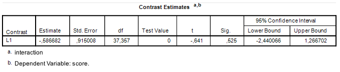
. Let’s use the results in Figure 1 to calculate what MOE is for this particular contrast.

#sample sizes per treatment
n = 12
m = 6

#obtained mean squares (see Figure 1): 
MSp = 6.403
MSs = 10.137
MSe = 1.470

#Relative error variance: 
VarT = (MSp + MSs - MSe) / (n*m)

#contrast weights: 
weights = c(1, -1, -1, 1)

#standard error of contrast estimate
SEcontrast = sqrt(sum(weights^2)*VarT)

#Satterthwaite degrees of freedom: 
dfp = 44
dfs = 20
dfe = 220
df = (MSp + MSs - MSe)^2 / (MSp^2/dfp + MSs^2/dfs + MSe^2/dfe)

#critical T 
critT = qt(.975, df)

#Margin of Error 
MOE = critT * SEcontrast

SEcontrast; MOE
## [1] 0.9149985
## [1] 1.853368

SPSS GLM Univariate uses the wrong standard error for a mixed model contrast estimate

Even though SPSS GLM Univariate allows you to specify a mixed model design and tests the treatment effect with a linear combination of mean squares, the procedure does not use the correct error variance if you want to estimate the value of a contrast (using the CONTRAST subcommand), it uses MSError instead. In our example, then, SPSS uses an error variance that is an order of magnitude smaller than the correct error variance: 1.47, with 220 degrees of freedom and not 15.07, with 37.357 (see Figure 1). The consequence of this is, of course, that the 95% CI is much narrower than it should be.

Running the syntax above Figure 1 gives the output in Figure 2. The results can be reproduced as follows. The standard error of the contrast is the result of SE = \sqrt{\sum{c_i^2}\frac{MSe}{nm}} = \sqrt{4*1.47/72} = 0.2858, the critical value of t is the .975 quantile of the central t distribution with df = 220, which equals 1.9708. The value of MOE is therefore MOE = 0.5633. With a contrast estimate of -0.587, the 95% CI equals -0.587 \pm 0.5633 = [-1.1503, -0.0237]. In comparison, using the correct value of MOE gives us [−2.4404, 1.2664].

Figure 2: SPSS GLM Univariate Contrasts Output
Thus, even though SPSS GLM Univariate gives us the ingredients to work with, i.e. an estimate of the error variance and approximate degrees of freedom, it should not be used for obtaining contrast estimates if you have a mixed model. SPSS Mixed does a much better job and the MIXED output also contains other useful data we can use for sample size planning. (In practice, I use the linear mixed effects modeling package LME4) and not so much SPSS). Have a quick look at Figure 3 for the contrast estimate obtained with the mixed procedure. (Note how the numbers are essentially the same as the ones we obtained when using the ANOVA source table of SPSS GLM Univariate (Figure 1)).
MIXED score BY cond   
/CRITERIA=CIN(95) MXITER(100) MXSTEP(10) SCORING(1) 
SINGULAR(0.000000000001) HCONVERGE(0, ABSOLUTE) 
LCONVERGE(0, ABSOLUTE) PCONVERGE(0.000001, ABSOLUTE)   
/FIXED= cond | SSTYPE(3)   
/METHOD=REML  
/TEST= 'interaction' cond 1 -1 -1 1   
/RANDOM=INTERCEPT | SUBJECT(pp) COVTYPE(VC)  
/RANDOM=INTERCEPT | SUBJECT(ss) COVTYPE(VC).
Figure 3: Contrast Estimate SPSS Mixed


Planning for precision

Even though the result in Figure 3 is hard to interpret without substantive detail (the data are made up) it is clear that the precision of the estimate is, well, suboptimal. As an indication: the estimated within treatment standard deviaion is about 1.74, so the estimated difference between differences (interaction) is close to a value of Cohen’s d of -.30, approximate 95% CI [-1.40, 0.73], which according to the rules of thumb is a medium negative effect, but consistent with anytihing from a huge negative effect to a large positive effect in the population, as the approximate CI shows. (I have divided the point estimate and the confidence interval in Figure 2 by 1.74, to obtain Cohen’s d and an approximate confidence interval). Clearly, then, our precision can be optimized.

Suppose that you are very fond of the both-within-condition design (BwC-design) and you plan to use it again in a replication study, You could of courseopt for a design with better expected precision, but based on the data and estimates at hand, that involves a lot of assumptions, but I will show you how you can do it in one of the next posts. If you plan for precision using the BwC-design, you need the following ingrediënts.

1. A figure for your target MOE. Let’s set target MOE to .40.

2. A specification of the percentage of assurance. Let’s say we want 80% assurance that target MOE will not exceed .40.

3. Estimates (or guesstimates) of the person variance \sigma^2_p, the stimulus variance \sigma^2_s, and the error variance \sigma^2_e. We will have a look in the next section.

4. Functions for calculating the relative error variance, degrees of freedom, MOE and determining the required sample sizes for Participants and Stimuli. These are all present in the Precision App, so I will use the application, but I will show how the results of the sample sizes relate to the information above.

Obtaining estimates of the variance components

We need to specify the values of three variance components. These variance components can be estimated on the basis of the mean squares and sample sizes obtained with SPSS GLM Univariate, we can use SPSS MIXED to obtain direct estimates or any other way to estimate variance components, such as GLM VARCOMPS (which has several estimation procedures). I like to use SPSS MIXED or LME4. and not a dedicated program for variance components, because most of the times the main purpose of the analysis I am doing is obtaining contrast estimate or F-tests, so most of the times variance components estimates are a handy by-product of my main analysis. For demonstrative purposes, I will show how it can be done with the GLM univariate output and I will show how the results match those of SPSS MIXED.

Take a look at Figure 1. The estimate of \sigma^2_e is simply MS(Error) = 1.47. For obtaining an estimate for the variance component associated with participants, we set the obtained mean square equal to the expected mean square (see Table 1). Thus, 6.403 = m\sigma^2_p + \sigma^2_e. Rearranging and using 1.47 as an estimate for \sigma^2_e leads to \sigma^2_p = (6.403 - \sigma^2_e) / m = (6.403 - 1.47) / 6 = 0.8222. Likewise, the estimate for \sigma^2_s = (10.137 - 1.47) / 12 = .7223. Thus, our estimates are \hat{\sigma}^2_e = 1.47, \hat{\sigma}^2_p = 0.8222, and \hat{\sigma}^2_s = 0.7223.

In order to obtain direct estimates you can use SPSS Mixed (or GLM Varcomps, or whatever you like). If you run the SPSS syntax in Figure 3, you will find estimates of the variance components under the heading Covariance Parameters in your SPSS output. See Figure 4. Note that the standard errors are pretty large, so the point estimates are not very precise. But since it is the only information we have, we will consider the point estimates to be the best we have.

Figure 4: Variance components estimates


Getting sample sizes with the Precision application

 
Let’s use the Precision app (https://gmulder.shinyapps.io/precision/) for sample size planning. Set the design to Stimulus and Participant within condition, the number of conditions to 4 and in the options for contrast 3 fill in the weights {1, -1, -1, 1} (Note: it is not necessary to fill it in in contrast 3).
 
For target MOE fill in 0.4, for assurance the value .80 and the values 1.47, 0.82, and 0.72 for, respectively, Residual variance, Participant intercept variance and Stimulus intercept variance. Fill in the value 0 for all the other variances. See Figure 5.
 
 
Figure 5: Setting values in the Precision App.
 
Press the button “Get Sample Sizes”. The calculations take a while, so make yourself some coffee (or anything else you like) and when you return the screen should show something like Figure 6a.
Figure 6a: Output for planning target MOE = 0.40
 
Figure 6b: Outpur for planning target MOE = 0.50
 
By the way, if you wonder why you can simply set the three interaction variance components to zero, then it may be nice to know that the variance components estimates obtained from the both-within-condition design already include them. For example, the estimate of the resiidual variance obtained with the both-within-condition design is actually the sum of the residual variance component and the interaction conponent of participant and stimulus. These latter components can only be separated in a fully-crossed-design where all participants respond to all stimuli in all conditions. Thus, if we use the symbol \sigma^2_{e, bwc}, to refer to the residual variance in the BwC-design, we can say \sigma^2_{e, bwc} = \sigma^2_{ps} + \sigma^2_e. Normally, the precision app sums these two components to get a value for the residual variance in the BwC-design, and you will obviously get the same result if you specify the residual variance as the sum and the participant-by-stimulus variance as 0. Likewise, \sigma^2_{p, bwc} = \sigma^2_p + \sigma^2_{cp}, and \sigma^2_{s, bwc} = \sigma^2_s + \sigma^2_{cs}, where \sigma^2_{cp} and \sigma^2_{cs} are the variances associated with the interaction of treatment and participant and treatment and stimulus, respectively.
 
If you look at the sample sizes in Figure 6a, you may notice that the numbers look odd. For example, the app says that the smallest number of stimuli is 877 but it also says that you only need 500 stimuli if you select 802 participants. And something like that happens to the participants as well. The output says that the smaller number of participants is 802, but it also suggest using 500 of them if you use 877 stimuli, which is clearly smaller than 802. To me this seems a little inconsistent. But I think I figured out what’s going on. The reason for these inconsistencies is that the application minimizes the sample sizes, but with a maximum of 500 for the other sample sizes. So, the smallest number of stimuli is 877 given that the maximum number of participants is 500. In other words, a smaller sample size is possible, but then we have to increase the maximum number of participants. In other words, in order to have 80% assurance to obtain a target MOE of no more than .40, we need at least 500 stimuli or at least 500 participants. If you look at Figure 6b, you will not notice these inconsistencies. The difference between the left and right sample sizes is that sizes on the right are based on a target MOE of .50 instead of .40.
 
According to Figure 6a, we can obtain our target if we use 802 participants and 500 stimuli. Since we are planning for an experiment with 4 treatment conditions, these total sample sizes need to be divided by 4 to get the sample sizes per treatment conditions. Thus, n = 804/4 = 201 participants, and m = 500 / 4 = 125 stimuli per treatment condition (I’ve increased the participants sample size to make it divisible by 4). For many experiments these numbers are impractically large, of course, so in this case you would probably either consider an alternative design or else you have to live with the message that you may not get the precision you want or need.
 

Checking the sample size suggestions using what we know

If we fill in the sample sizes (802 participants and 500 stimuli) in the Precision app we get the results presented in Figure 7 for the interaction contrast (contrast 3). Expected MOE equals 0.3927, and there is 80% assurance that MOE will not exceed 0.4065
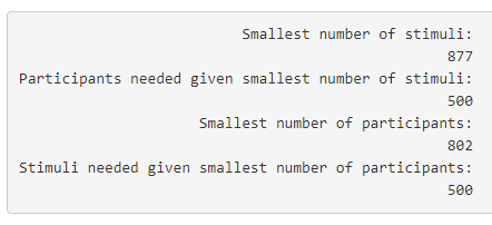
. Note, again, that the assurance MOE is somewhat larger than target MOE, because a sample of 804 participants requires a sample of more than 500 stimuli to get the target MOE with 80% assurance and 500 stimuli is the maximum number of stimuli the app considers when minimizing the number of participants.
 
Figure 7: Expected and Assurance MOE for the interaction contrast (contrast 3) using 804 participants and 500 stimuli
Let’s see if we can reconstruct the figures using what we know from previous sections. First the relative error variance of the treatment mean. That relative error variance is (m\sigma^2_p + n\sigma^2_s + \sigma^2_e)/ nm = 0.0099.
 
The degrees of freedom can be calculated by first filling in the expected mean squares and the degrees of freedom presented in Table 1: MS_p = 125*.82 + 1.47 = 103.96, df_p = 800, MS_s = 201*.72 + 1.47 = 146.19, df_s = 496, MS_e = 1.47, and df_e = 4*(201 - 1)*(125 - 1) = 99200. The Satterthwaite degrees of freedom are (MS_p + MS_s - MS_e)^2 / (MS_p^2/df_p + MS_s^2/df_s + MS_e^2/df_e) = 1092.66. The standard error of the contrast equals \sqrt{4*.0099} = 0.1990. The critical value for t equals 1.9621. Expected MOE is, therefore, 0.3905 (the tiny difference with the results from the app is due to rounding errors).
 
For the calculation of assurance MOE we need to take the sampling distribution of the relative error variance of the treatment mean into account. The app uses the (scaled) \chi^2-distribution. That is, we assume with assurance \gamma, that the \gamma quantile of the sampling distribution of the relative error error variance is \sigma^2_{\bar{X}, rel}*\chi^2_{\gamma, df}/df. Now, the degrees of freedom are 1092.66, the assurance \gamma = .80, and the .80 quantile of \chi^2 with 1092.66 degrees of freedom equals 1131.7966. Since the relative error variance equals 0.0099, the .80 quantile of the error variance equals 0.0099*1131.7966/1092.66 = 0.0103. And this means that assurance MOE equals 1.9621*\sqrt{4*0.0103} = 0.3982. Again, the difference with the results from the Precision App are due to rounding error.

Planning for a precise slope estimate in simple regression

In this post, I will show you a way of determining a sample size for obtaining a precise estimate of the slope \beta_1of the simple linear regression equation \hat{Y_i} = \beta_0 + \beta_1X_i. The basic ingredients we need for sample size planning are a measure of the precision, a way to determine the quantiles of the sampling distribution of our measure of precision, and a way to calculate sample sizes.

As our measure of precision we choose the Margin of Error (MOE), which is the half-width of the 95% confidence interval of our estimate (see: Cumming, 2012; Cumming & Calin-Jageman, 2017; see also www.thenewstatistics.com).

The distribution of the margin of error of the regression slope

In the case of simple linear regression, assuming normality and homogeneity of variance, MOE is t_{.975}\sigma_{\hat{\beta_1}}, where t_{.975}, is the .975 quantile of the central t-distribution with N - 2 degrees of freedom, and \sigma_{\hat{\beta_1}} is the standard error of the estimate of \beta_1.
An expression of the squared standard error of the estimate of \beta_1 is \frac{\sigma^2_{Y|X}}{\sum{(X_i - \bar{X})}^2} (Wilcox, 2017): the variance of Y given X divided by the sum of squared errors of X. The variance \sigma^2_{Y|X} equals \sigma^2_y(1 - \rho^2_{YX}), the variance of Y multiplied by 1 minus the squared population correlation between Y and X, and it is estimated with the residual variance \frac{\sum{(Y -\hat{Y})^2}}{df_e}, where df_e = N - 2.
The estimated squared standard error is given in (1)

(1)   \[\hat{\sigma}_{\hat{\beta_{1}}}^{2}=\frac{\sum(Y-\hat{Y})^{2}/df_{e}}{\sum(X-\bar{X})^{2}}. \]

With respect to the sampling distribution of MOE, we first note the following. The distribution of estimates of the residual variance in the numerator of (1) is a scaled \chi^2-distribution:

    \[\frac{\sum(Y-\hat{Y})^{2}}{\sigma_{y}^{2}(1-\rho^{2})}\sim\chi^{2}(df_{e}),\]

thus

    \[\frac{\sum(Y-\hat{Y})^{2}}{df_{e}}\sim\frac{\sigma_{y}^{2}(1-\rho^{2})\chi^{2}(df_{e})}{df_{e}}.\]

Second, we note that

    \[\frac{\sum(X-\bar{X})^{2}}{\sigma_{X}^{2}}\sim\chi^{2}(df),\]

where df = N - 1, therefore

    \[\sum(X-\bar{X})^{2}\sim\sigma_{X}^{2}\chi^{2}(df).\]

Alternatively, since \sum{(X - \bar{X})^2} = df\sigma^2_X, and multiplying by 1 (\frac{df}{df}).

    \[df\sigma_{X}^{2}\sim df\sigma_{X}^{2}\chi^{2}(df)/df.\]

In terms of the sampling distribution of (1), then, we have the ratio of two (scaled) \chi^2 distributions, one with df_e = N - 2 degrees of freedom, and one with df = N - 1 degrees of freedom. Or something like:

    \[\hat{\sigma}_{\hat{\beta_{1}}}^{2}\sim\frac{\sigma_{y}^{2}(1-\rho^{2})\chi^{2}(df_{e})/df_{e}}{df\sigma_{X}^{2}\chi^{2}(df)/df}=\frac{\sigma_{y}^{2}(1-\rho^{2})}{df\sigma_{X}^{2}}\frac{\chi^{2}(df_{e})/df_{e}}{\chi^{2}(df)/df}=\frac{\sigma_{y}^{2}(1-\rho^{2})F(df_{e,}df)}{df\sigma_{X}^{2}},\]

which means that the sampling distribution of MOE is:

(2)   \[\hat{MOE}\sim t_{.975}(N-2)\sqrt{\frac{\sigma_{y}^{2}(1-\rho^{2})F(N-2,N-1)}{(N-1)\sigma_{X}^{2}}}. \]

This last equation, that is (2), can be used to obtain quantiles of the sampling distribution of MOE, which enables us to determine assurance MOE, that is the value of MOE that under repeated sampling will not exceed a target value with a given probability. For instance, if we want to know the .80 quantile of estimates of MOE, that is, assurance is .80, we determine the .80 quantile of the (central) F-distribution with N – 2 and N – 1 degrees of freedom and fill in (2) to obtain a value of MOE that will not be exceeded in 80% of replication experiments.
For instance, suppose \sigma^2_Y = 1, \sigma^2_X = 1, \rho = .50, N = 100, and assurance is .80, then according to (2), 80% of estimated MOEs will not exceed the value given by:
vary = 1
varx = 1
rho = .5
N = 100 
dfe = N - 2
dfx - N - 1
assu = .80
t = qt(.975, dfe)
MOE.80 = t*sqrt(vary*(1 - rho^2)*qf(.80, dfe, dfx)/(dfx*varx))
MOE.80
## [1] 0.1880535

What does a quick simulation study tell us?

A quick simulation study may be used to check whether this is at all accurate. And, yes, the estimated quantile from the simulation study is pretty close to what we would expect based on (2). If you run the code below, the estimate equals 0.1878628.
library(MASS)
set.seed(355)
m = c(0, 0)

# note: s below is the variance-covariance matrix. In this case,
# rho and the cov(y, x) have the same values
# otherwise: rho = cov(x, y)/sqrt(varY*VarX) (to be used in the 
# functions that calculate MOE)
# equivalently, cov(x, y) = rho*sqrt(varY*varX) (to be used
# in the specification of the variance-covariance matrix for 
#generating bivariate normal variates)

s = matrix(c(1, .5, .5, 1), 2, 2)
se <- rep(10000, 0)
for (i in 1:10000) {
theData <- mvrnorm(100, m, s)
mod <- lm(theData[,1] ~ theData[,2])
se[i] <- summary(mod)$coefficients[4]
}
MOE = qt(.975, 98)*se
quantile(MOE, .80)
##       80% 
## 0.1878628

Planning for precision

If we want to plan for precision we can do the following. We start by making a function that calculates the assurance quantile of the sampling distribution of MOE described in (2). Then we formulate a  squared cost function, which we will optimize for the sample sizeusing the optimize function in R.
Suppose we want to plan for a target MOE of .10 with 80% assurance.We may do the following.
vary = 1
varx = 1
rho = .5
assu = .80
tMOE = .10

MOE.assu = function(n, vary, varx, rho, assu) {
        varY.X = vary*(1 - rho^2)
        dfe = n - 2
        dfx = n - 1
        t = qt(.975, dfe)
        q.assu = qf(assu, dfe, dfx)
        MOE = t*sqrt(varY.X*q.assu/(dfx * varx))
        return(MOE)
}

cost = function(x, tMOE) { 
cost = (MOE.assu(x, vary=vary, varx=varx, rho=rho, assu=assu) 
- tMOE)^2
}

#note samplesize is at least 40, at most 5000. 
#note that since we already know that N = 100 is not enough
#in stead of 40 we might just as well set N = 100 at the lower
#limit of the interval
(samplesize = ceiling(optimize(cost, interval=c(40, 5000), 
tMOE = tMOE)$minimum))
## [1] 321
#check the result: 
MOE.assu(samplesize, vary, varx, rho, assu)
## [1] 0.09984381

Let’s simulate with the proposed sample size

Let’s check it with a simulation study. The value of estimated .80 of estimates of MOE is 0.1007269 (if you run the below code with random seed 335), which is pretty close to what we would expect based on (2).
set.seed(355)
m = c(0, 0)

# note: s below is the variance-covariance matrix. In this case,
# rho and the cov(y, x) have the same values
# otherwise: rho = cov(x, y)/sqrt(varY*VarX) (to be used in the 
# functions that calculate MOE)
# equivalently, cov(x, y) = rho*sqrt(varY*varX) (to be used
# in the specification of the variance-covariance matrix for 
# generating bivariate normal variates)

s = matrix(c(1, .5, .5, 1), 2, 2)
se <- rep(10000, 0)
samplesize = 321
for (i in 1:10000) {
theData <- mvrnorm(samplesize, m, s)
mod <- lm(theData[,1] ~ theData[,2])
se[i] <- summary(mod)$coefficients[4]
}
MOE = qt(.975, 98)*se
quantile(MOE, .80)
##       80% 
## 0.1007269

References

Cumming, G. (2012). Understanding the New Statistics. Effect Sizes, Confidence Intervals, and Meta-Analysis. New York: Routledge
Cumming, G., & Calin-Jageman, R. (2017). Introduction to the New Statistics: Estimation, Open Science, and Beyond. New York: Routledge.
Wilcox, R. (2017). Understanding and Applying Basic Statistical Methods using R. Hoboken, New Jersey: John Wiley and Sons.