
In this post, I illustrate how to do contrast analysis for within subjects designs with R. A within subjects design is also called a repeated measures design. I will illustrate two approaches. The first is to simply use the one-sample t-test on the transformed scores. This will replicate a contrast analysis done with SPSS GLM Repeated Measures. The second is to make use of mixed linear effects modeling with the lmer-function from the lme4 library.
Conceptually, the major difference between the two approaches is that in the latter approach we make use of a single shared error variance and covariance across conditions (we assume compound symmetry), whereas in the former each contrast has a separate error variance, depending on the specific conditions involved in the contrast (these conditions may have unequal variances and covariances).
As in the previous post (https://small-s.science/2018/12/contrast-analysis-with-r-tutorial/), we will focus our attention on obtaining an interaction contrast estimate.
Again, our example is taken from Haans (2018; see also this post). It considers the effect of students’ seating distance from the teacher and the educational performance of the students: the closer to the teacher the student is seated, the higher the performance. A “theory “explaining the effect is that the effect is mainly caused by the teacher having decreased levels of eye contact with the students sitting farther to the back in the lecture hall.
To test that theory, a experiment was conducted with N = 9 participants in a completely within-subjects-design (also called a fully-crossed design), with two fixed factors: sunglasses (with or without) and location (row 1 through row 4). The dependent variable was the score on a 10-item questionnaire about the contents of the lecture. So, we have a 2 by 4 within-subjects-design, with n = 9 participants in each combination of the factor levels.
We will again focus on obtaining an interaction contrast: we will estimate the extent to which the difference between the mean retention score on the first row and those on the other rows differs between the conditions with and without sunglasses.
Contrast Analysis with SPSS Repeated Measures
I’ve downloaded a dataset from the supplementary materials accompanying Haans (2018) from http://pareonline.net/sup/v23n9.zip (Within2by4data.sav) and I ran the following syntax in SPSS:
GLM noglasses_row1 noglasses_row2 noglasses_row3 noglasses_row4
glasses_row1 glasses_row2 glasses_row3 glasses_row4
  /WSFACTOR=sunglasses 2 location 4
  /MMATRIX = "Interaction contrast"
  ALL 1 -1/3 -1/3 -1/3 -1 1/3 1/3 1/3
  /MEASURE=Retention
  /METHOD=SSTYPE(3)
  /CRITERIA=ALPHA(.05)
  /WSDESIGN=sunglasses location sunglasses*location.
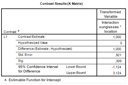
The relevant output for our purposes is:
 |
| SPSS interaction contrast repeated measures |
The estimated value of the interaction contrasts equals 1.00, 95% CI [-1.12, 3.12]. (With a p-value of p = .309).
Contrast analysis for within subjects designs with R
The following code can be used replicate the SPSS results if we do contrast analysis for within subjects designs with R.
library(foreign)

theData <- as.data.frame(read.spss(file="./Within2by4data.sav"))

myContrast = c(1, -1/3, -1/3, -1/3, -1, 1/3, 1/3, 1/3)

transformedScores = as.matrix(theData[,-1]) %*% myContrast

t.test(transformedScores)
##
##  One Sample t-test
##
## data:  transformedScores
## t = 1.0854, df = 8, p-value = 0.3093
## alternative hypothesis: true mean is not equal to 0
## 95 percent confidence interval:
##  -1.124486  3.124486
## sample estimates:
## mean of x
##         1
Let me walk you through it.
On the first line, we load the foreign package so that we can read the SPSS data-file with the read.spss function we call on the second line of our code. The third line specifies the interaction contrast. On the fourth line we create the variable transformedScores by calculating the inner product of the 8 observations per participant and the contrast weights (theData[, -1] is the data without the first column containing the participant id). The result is a (column) vector of contrast scores (one per participant). On the last line, we use the t.test-function to obtain a one-sample t-test, testing the null-hypothesis that the mean contrast score (transformed score) is equal to zero.
The result show that the contrast estimate equals 1.00, 95% CI [-1.12, 3.12] (t(8) = 1.09, p = .31).
Obtaining the interaction contrast with SPSS mixed
If we want to make use of the model assumptions of equal variances and covariances we can opt for a linear mixed model. I’ve transformed Haans’ (2018) data from wide to long format (if you need to do that with your own dataset, take a look here; you can download my file here: download the spss file).
MIXED retention BY sunglasses location
  /CRITERIA=CIN(95) MXITER(100) MXSTEP(10) SCORING(1)
SINGULAR(0.000000000001) HCONVERGE(0, ABSOLUTE) LCONVERGE(0, ABSOLUTE)
PCONVERGE(0.000001, ABSOLUTE)
  /FIXED=sunglasses location sunglasses*location | SSTYPE(3)
 /TEST "Interaction" sunglasses*location 1 -1/3 -1/3 -1/3 -1 1/3 1/3 1/3
  /METHOD=REML
  /RANDOM=INTERCEPT | SUBJECT(person) COVTYPE(CS).
The relevant output is the following.

The result show that the contrast estimate equals 1.00, 95% CI [-0.24, 2.24] (t(56) = 1.62, p = .11).
The interaction contrast with R, lme4 and Emmeans
The analysis above can be replicated in R as follows.
library(lme4)
library(emmeans)

theData <- as.data.frame(read.spss(file="./Within2by4dataLong.sav"))

theData$person <- factor(theData$person)

attach(theData)

myMod <- lmer(retention ~ sunglasses*location + (1|person))

myContrast = c(1, -1/3, -1/3, -1/3, -1, 1/3, 1/3, 1/3)

condMeans <- emmeans(myMod, ~location*sunglasses)

contrast(condMeans, list("interaction"= myContrast))
##  contrast    estimate       SE df t.ratio p.value
##  interaction        1 0.618284 56   1.617  0.1114
# confidence interval

1 + c(-qt(.975, 56), qt(.975, 56))*.618284
## [1] -0.2385717 2.2385717
Alternatively, set emmeans options to obtain confidence intervals for the estimates:
emm_options(contrast = list(infer=c(TRUE, FALSE)))
contrast(condMeans, list("interaction"= myContrast))
##  contrast    estimate       SE df   lower.CL upper.CL
##  interaction        1 0.618284 56 -0.2385717 2.238572
##
## Confidence level used: 0.95
Or to get both an interval and a p-value:
emm_options(contrast = list(infer=c(TRUE, TRUE)))
contrast(condMeans, list("interaction"= myContrast))
##  contrast    estimate       SE df   lower.CL upper.CL t.ratio p.value
##  interaction        1 0.618284 56 -0.2385717 2.238572   1.617  0.1114
##
## Confidence level used: 0.95
Reference
Haans, Antal (2018). Contrast Analysis: A Tutorial. Practical Assessment, Research, & Education, 23(9). Available online: http://pareonline.net/getvn.asp?v=23&n=9