Both theory underlying the Precision application and the use of the app in practice rely for a large part on specifying variance components. In this post, I will give you some more details about what these components are, and how they relate to the analysis of variance model underlying the app.
What is variance?
As you probably know, the normal distribution is centered around its mean value, which is (equal to) the parameter μ. We call this parameter the population mean.
Now, we select a single random value from the population. Let’s call this value X. Because we know something about the probability distribution of the population values, we are also in the position to specify an expected value for the score X. Let’s use the symbol E(X) for this expected value. The value of E(X) proves (and can be proven) to be equal to the parameter μ. (Conceptually, the expectation of a variable can be considered as its long run average).
Of course, the actual value obtained will in general not be equal to the expected value, at least not if we sample from continuous distributions like the normal distribution. Let’s call the difference between the value X and it’s expectation E(X) = μ. an error, deviation or residual: e = X – E(X) = X – μ.
We would like to have some indication of the extent to which X differs from its expectation, especially when E(X) is estimated on the basis of a statistical model. Thus, we would like to have something like E(X – E(X)) = E(X – μ). The variance gives us such an indication, but does so in squared units, because working with the expected error itself always leads to the value 0 E(X – μ) = E(X) – E( μ) = μ – μ = 0. (This simply says that on average the error is zero; the standard explanation is that negative and positive errors cancel out in the long run).
The variance is the expected squared deviation (mean squared error) between X and its expectation: E((X – E(X))2) = E(X – μ)2), and the symbol for the population value is σ2.
Some examples of variances (remember we are talking conceptually here):
– the variance of the mean, is the expected squared deviation between a sample mean and its expectation the population mean.
– the variance of the difference between two means: the expected squared deviation between the sample difference and the population difference between two means.
– the variance of a contrast: the expected squared deviation between the sample value of the contrast and the population value of the contrast.
It’s really not that complicated, I believe.
Note: in the calculation of t-tests (and the like), or in obtaining confidence intervals, we usually work with the square root of the variance: the root mean squared error (RMSE), also known as the standard deviation (mostly used when talking about individual scores) or standard error (when talking about estimating parameter values such as the population mean or the differences between population means).
What are variance components?
In order to appreciate what the concept of a variance component entails, imagine an experiment with nc treatment conditions in which np participants respond to ni items (or stimuli) in all conditions. This is called a fully-crossed experimental design.
Now consider the variable Xcpi. a random score in condition t, of participant p responding to item i. The variance of this variable is σ2(Xcpi) = E((Xcpi – μ)2). But note that just as the single score is influenced by e.g. the actual treatment condition, the particular person or item, so too can this variance be decomposed into components reflecting the influence of these factors. Crucially, the total variance σ2(Xcpi) can be considered as the sum of independent variance components, each reflecting the influence of some factor or interaction of factors.
The following figure represents the components of the total variance in the fully crossed design (as you can see the participants are now promoted to actual persons…)
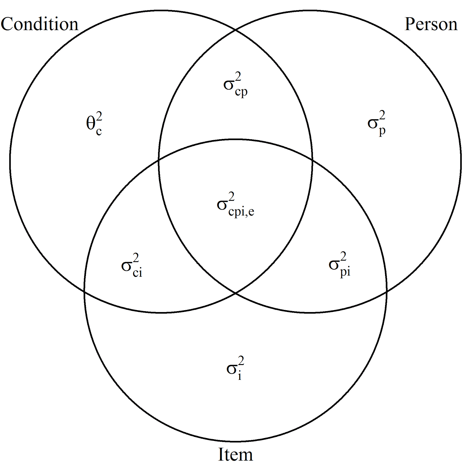
The symbols used in this figure represent the following. Θ2 is used to indicate that a component is considered to be a so-called fixed variance component (the details of which are beyond the scope of this post), and the symbol σ2 is used to indicate components associated with random effects. (The ANOVA model contains a mixture of fixed and random effects, that’s why we call such models mixed effects models or mixed model ANOVAs). Components with a single subscript represent variances associated with main effects, components with two subscripts two-way interactions, and the only component with three subscripts represents a three-way-interaction confounded with error.
Let’s consider one of these variance components (you can also refer to them simply as variances) to see in more detail how they can be interpreted. Take σ2(p), the person-variance. Note that this is an alternative symbol for the variance, in the figure, the p is in the subscript in stead of between brackets (I am sorry for the inconvenience of switching symbols, but I do not want to rely too much on mathjax ($sigma^2_p = sigma^2(p)$) and I do not want to change the symbols in the figure).
The variance σ2(p) is the expected squared deviation of the score of an idealized randomly selected person and the expectation of this score, the population mean. This score is the person score averaged of the conditions of the experiment and all of the items that could have been selected for the experiment. (This conceptualization is from Generalizability Theory; the Venn-diagram representation as well), the person score is also called the universe score of the person).
The component represents E((μp – μ)2), the expected squared person effect. Likewise, the variance associated with items σ2(i) is the expected squared item effect, and σ2(cp), is the expected squared interaction effect of condition and person.
The figure indicates that the total variance is (modeled as) the sum of seven independent variance components. The Precision app asks you to supply the values for six of these components (the components associated with the random effects), and now I hope it is a little clearer why these components are also referred to as expected squared effects.
Relative error variance of a treatment mean
But these components specify the variance in terms of individual measurements, whereas the treatment mean is obtained on the basis of averaging over the np*ni measurements we have in the corresponding treatment condition. So let’s see how we can take into account the number of measurements.
Unfortunately, things get a little complicated to explain, but I’ll have a go nonetheless. The explanation takes two steps: 1) We consider how to specify expected mean squares in terms of the components contained in the condition-circle 2) We’ll see how to get from the formulation of the expected mean square to the formulation of the relative error variance of a treatment mean.
Obtaining an expected mean square
I will use the term Mean Square (MS) to refer to a variance estimate. For instance, MST is an estimate of the variance associated with the treatment condition. The expected MS (EMS) is the average value of these estimates.
We can use the Venn-diagram to obtain an EMS for the treatment factor and all the other factors in the design, but we will focus on the EMS associated with treatment. However, we cannot use the variance components directly, because the mixed ANOVA model I have been using for the application contains sum-to-zero restrictions on the treatment effects and the two-way interaction-effects of treatment and participant and treatment and stimulus (item). The consequence of this is that we will have to multiply the variance components associated with the treatment-by-participant and treatment-by-stimulus with a constant equal to nc / (nc – 1), where nc is the number of conditions.(This is the hard part to explain, but I didn’t really explain it, but simply stated it).
The second step of obtaining the EMS is to multiply the components with the number of participants and items, as follows. Multiply the component by the sample size if and only if the subscript of the component does not contain a reference to the particular sample size. That is, for instance, multiply a component by the number of participants np, if and only if the subscript of the component does not contain a subscript associated with participants.
This leads to the following:
E(MST) = npniΘ2(T) + ni(nc / (nc – 1))σ2(cp) + np(nc / (nc – 1))σ2(ci) + σ2(cpi, e).
Obtaining the relative error variance of the treatment mean
Notice that ni(nc / (nc – 1))σ2(cp) + np(nc / (nc – 1))σ2(ci) + σ2(cpi, e) contains the components associated with the relative error variance. Because the treatment mean is based on np*ni scores, to obtain the relative error variance for the treatment mean, we divide by np*ni to obtain.
Relative error variance of the treatment mean = (nc / (nc – 1))σ2(cp) / np + (nc / (nc – 1))σ2(ci) / ni+ σ2(cpi, e) / (npni).
As an aside, in the post describing the app, I have used the symbols σ2(αβ) to refer to nc / (nc – 1))σ2(cp), and σ2(αγ) to refer to (nc / (nc – 1))σ2(ci).
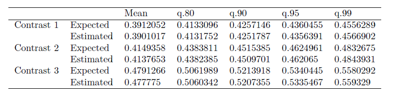
Comparing means: the error variance of a contrast
Note that the latter gives us the expected squared deviation between the estimated contrast value and the true contrast value (see also the explanation of the concept of variance above).
It should be noted that for the calculation of a 95% confidence interval for the contrast estimate (or for the Margin of Error; the half-width of the confidence interval) we make use of the square root of the error variance of the contrast. This square root is the standard error of the contrast estimate. The calculation of MOE also requires a value for the degrees of freedom. I will write about forming a confidence interval for a contrast estimate in one of the next posts.