Tutorials Archives - The small S scientist

May 22, 2022May 22, 2022

The independent and paired T-test in jamovi

This is a short tutorial on comparing two means with the independent and paired t-test in jamovi.

Description of the data

I have downloaded the dataset from the Mathematics and Statistics Help (MASH) site. The dataset contains data on 78 persons following one of three diets. I will use the dataset to show you how to estimate the difference between two means with the independent t-test analysis and the dependent t-test analysis in jamovi. I will ignore the different diets and focus on gender differences and pre- and post-weight differences instead.

I will focus on two substantive research questions.

To what extent does following a diet lead to weight loss?
To what extent does the weight lost differ between females and males?

The paired t-test in jamovi

Let’s start with the first research question. Statistical analysis can be useful for answering the research question, but then we will first have to translate the substantive question into a statistical one. Now, it seems reasonable to assume that if following a diet leads to weight loss, that the typical weight before the diet differs from the typical weight after following the diet. If we assume furthermore that the mean provides a good representation of what is typical, then it is plausible that the mean weight before the diet differs from the mean weight after the diet.

If we are interested in the extent to which means differ, we are – statistically speaking – interested in the extent to which expected values differ. So, our analysis will focus on finding out what our data have to say about the difference between the expected values. More concrete: we focus on the difference between the expected values for weight (measured in kg) before and after the diet. Using conventional symbols, we aim at uncovering quantitative information about the difference $\mu_{pre\ weight} – \mu_{post\ weight}$ .

Since all persons were measured pre and post diet, the measurements are likely to be correlated. Indeed, the sample correlation equals r = .96. We need to take this correlation into account and that is why we use the statistical techniques for estimation and testing that are available in the paired t-test analysis in jamovi.

Doing the paired t-test in jamovi

In a real research situation, we would of course start with descriptive analyses to figure out what the data seem to suggest about the extent to which a diet leads to weight loss. But now we are just looking at how to obtain the relevant inferential information from jamovi.

I have chosen the following options for the analysis.

Choosing Jamovi paired t-test options — Figure 1. Paired t-test analysis options in jamovi

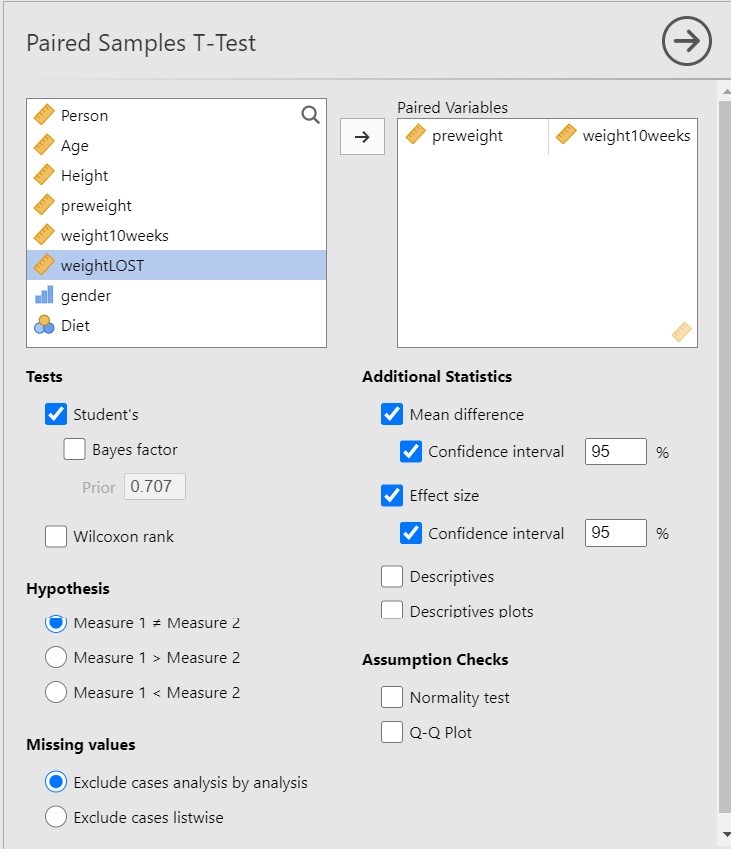
Since we are interested in the extent to which following a diet leads to weight loss, it is important to realize that the t-test in itself does not necessarily provide useful information. Why? Because the t-test gives us input to make the decision whether to reject the null-hypothesis that the expected values are equal, and only indirectly provides us with the information about the extent to which the expected values differ, and the latter is of course what we are interested in: we want quantitative information! The more useful information is provided by the estimate of the mean difference and the 95% Confidence Interval.

The paired t-test output

The relevant output for the t-test and the estimation results are presented in Figure 2.

Jamovi paired t-test output — Figure 2. Significance test and estimation results of the paired t-test analysis in jamovi

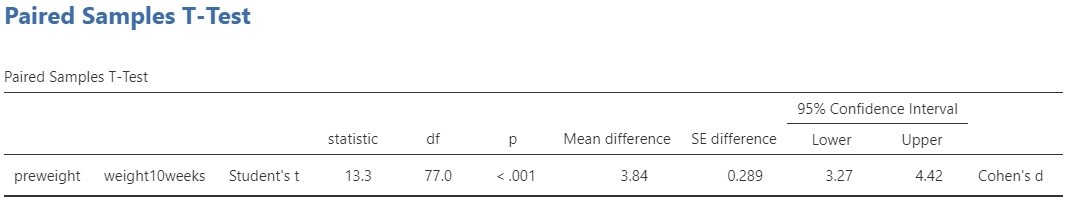
Let’s start with the t-test. The conventional null-hypothesis is that the expected values of the two variables are equal ( $\mu_{pre\ weight} = \mu_{post\ weight}$ , or $\mu_{pre\ weight} – \mu_{post\ weight} = 0.$ . The alternative hypothesis is that the expected values are not equal. Following convention, we use a significance level of $\alpha = .05$ , so that our decision rule is to reject the null-hypothesis if the p-value is smaller than .05 and to not reject but also not accept the null-hypothesis if the p-value is .05 or larger.

The result of the t-test is t(77) = 13.3, p < .001. Since the p-value is smaller than .05 we reject the null-hypothesis and we decide that the expected values are not equal. In other words, we decide that the population means are not equal. As we said above, this does not answer our research question, so we’d better move on to the estimation results.

The estimated difference between the expected values equals 3.84 kg, 95% CI [3.27, 4.42]. So, we estimate that the difference in expected weights after 10 weeks of following the diet is somewhere between 3.72 and 4.42 kilograms.

Cohen’s d for the paired design

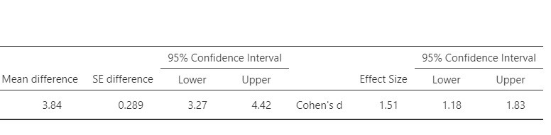
Jamovi also provides point and interval estimates for Cohen’s d. This version of Cohen’s d is derived by standardizing the mean difference using the standard deviation of the difference scores. Figure 3 presents the relevant output. The estimated value of Cohen’s delta equals 1.51, 95% CI [1.18, 1.83]. Using rules of thumb for the interpretation of Cohen’s d, these results suggest that there may be a very large difference in mean weights of the pre- and postdiet measurements.

Figure 3. Estimation results from the paired t-test analysis in jamovi

There is an alternative conceptualisation of the standardized mean difference. Instead of using the SD of the difference scores, we may use the average of the SDs of the two measurements. See https://small-s.science/2020/12/cohens-d-for-paired-designs/ for an explanation and R-code for the calculation of the CI.

The independent t-test in jamovi

To answer the second research question, we will have to reframe the substantive question into a statistical one. Just like we assumed above, we will consider the difference between the expected values (or population means) to be the statistical quantity of interest.

The conventional statistical null-hypothesis of the t-test is that the expected value of the variable does not differ between the groups or conditions. In other words, the null-hypothesis is that the two population means are equal. If the test result is significant, we will reject the null-hypothesis and decide that the population means are not equal. Note that this does not really answer the research question. Indeed, we are interested in the extent to which the expected values differ and not in whether we can decide that the difference is not zero. For that reason, estimation results are usually more informative than the results of a significance test.

Doing the independent t-test in jamovi.

I have chosen the following options for the independent t-test analysis in jamovi.

Options for the independent t-test in jamovi. — Figure 4. Options for the independen t-test in jamovi

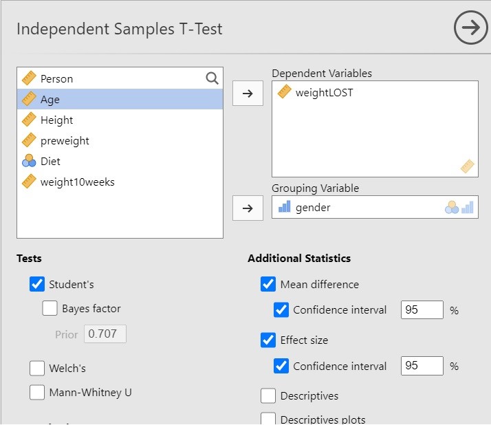
The above options will give you the results of the independent t-test and, more importantly, the estimation results, both unstandardized and standardized (Cohen’s d).

The independent t-test output

The relevant output is presented in Figure 5.

Output of the independent t-test analysis in jamovi. Including significance test and estimation results. — Figure 5. Output of the independent t-test analysis in jamovi

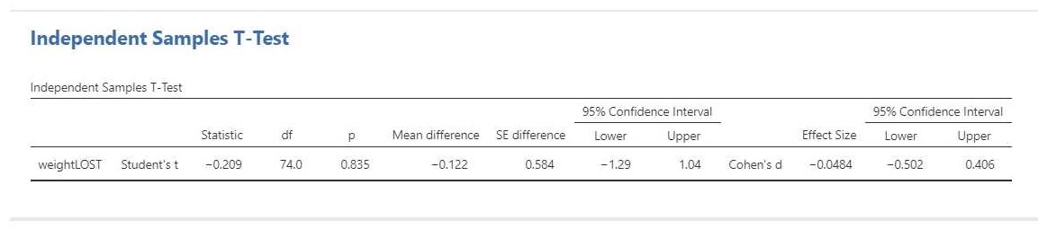
The result of the t-test is t(74) = -0.21, p = 0.84. This test result is clearly not significant, so we cannot decide that the population means differ. Importantly, we can also not decide that the population means are equal. That would be an instance of accepting the null-hypothesis and that is not allowed in NHST.

The estimation results (i.e. -0.12 kg, 95% CI [-1.29, 1.04]) make it clear that we should not necessarly believe that the population means are equal. Indeed, even though the estimated difference is only 0.12 kilograms, the CI shows the data to be consistent with differences up to 1 kg in either direction, i.e. with women showing more average weight loss than men or women showing less average weight loss than men.

Cohen’s d for the independent design

We can also find the standardized mean difference and its CI in the independent t-test output: Cohen’s d = -0.08, 95% CI [-0.50, 0.41]. In this case, Cohen’s d is based on the pooled standard deviaton. According to rules-of-thumb that are used frequently in psychology the estimated effect is negligible to small, but the CI shows the data to be consistent with medium effect sizes in either direction.

August 26, 2019December 8, 2020

Linear Trend Analysis with R and SPSS

This is an introduction to contrast analysis for estimating the linear trend among condition means with R and SPSS . The tutorial focuses on obtaining point and confidence intervals. The contents of this introduction is based on Maxwell, Delaney, and Kelley (2017) and Rosenthal, Rosnow, and Rubin (2000). I have taken the (invented) data from Haans (2018). The estimation perspective to statistical analysis is aimed at obtaining point and interval estimates of effect sizes. Here, I will use the frequentist perspective of obtaining a point estimate and a 95% Confidence Interval of the relevant effect size. For linear trend analysis, the relevant effect size is the slope coefficient of the linear trend, so, the purpose of the analysis is to estimate the value of the slope and the 95% confidence interval of the estimate. We will use contrast analysis to obtain the relevant data.

[Note: A pdf-file that differs only slightly from this blogpost can be found on my Researchgate page: here; I suggest Haans (2018) for an easy to follow introduction to contrast analysis, which should really help understanding what is being said below].

The references cited above are clear about how to construct contrast coefficients (lambda coefficients) for linear trends (and non-linear trends for that matter) that can be used to perform a significance test for the null-hypothesis that the slope equals zero. Maxwell, Delaney, and Kelley (2017) describe how to obtain a confidence interval for the slope and make clear that to obtain interpretable results from the software we use, we should consider how the linear trend contrast values are scaled. That is, standard software (like SPSS) gives us a point estimate and a confidence interval for the contrast estimate, but depending on how the coefficients are scaled, these estimates are not necessarily interpretable in terms of the slope of the linear trend, as I will make clear
momentarily.

So our goal of the data-analysis is to obtain a point and interval estimate of the slope of the linear trend and the purpose of this contribution is to show how to obtain output that is interpretable as such.

Continue reading “Linear Trend Analysis with R and SPSS”

April 14, 2019October 22, 2019

Planning for Precise Contrast Estimates: Introduction and Tutorial (Preprint)

I just finished a preprint of an introduction and tutorial to sample size planning for precision of contrast estimates. The tutorial focuses on single factor between and within subjects designs, and mixed factorial designs with one within and one between factor. The tutorial contains R-code for sample size planning in these designs.

The preprint is availabe on researchgate: Click (but I am just as happy to send it to you if you like; just let me know).

April 4, 2019October 22, 2019

Contrast analysis with R: Tutorial for factorial mixed designs

In this tutorial I will show how contrast estimates can be obtained with R. Previous posts focused on the analyses in factorial between and within designs, now I will focus on a mixed design with one between participants factor and one within participants factor. I will discuss how to obtain an estimate of an interaction contrast using a dataset provided by Haans (2018).

I will illustrate two approaches, the first approach is to use transformed scores in combination with one-sample t-tests, and the other approach uses the univariate mixed model approach. As was explained in the previous tutorial, the first approach tests each contrast against it’s own error variance, whereas in the mixed model approach a common error variance is used (which requires statistical assumptions that will probably not apply in practice; the advantage of the mixed model approach, if its assumptions apply, is that the Margin of Error of the contrast estimate is somewhat smaller).

Again, our example is taken from Haans (2018; see also this post. It considers the effect of students’ seating distance from the teacher and the educational performance of the students: the closer to the teacher the student is seated, the higher the performance. A “theory “explaining the effect is that the effect is mainly caused by the teacher having decreased levels of eye contact with the students sitting farther to the back in the lecture hall. To test that theory, a experiment was conducted with N = 9 participants in a factorial mixed design (also called a split-plot design), with two fixed factors: the between participants Sunglasses (with or without), and the within participants factor Location (row 1 through row 4). The dependent variable was the score on a 10-item questionnaire about the contents of the lecture. So, we have a 2 by 4 mixed factorial design, with n = 9 participants in each combination of the factor levels.

We will again focus on obtaining an interaction contrast: we will estimate the extent to which the difference between the mean retention score on the first row and those on the other rows differs between the conditions with and without sunglasses.

Continue reading “Contrast analysis with R: Tutorial for factorial mixed designs”

January 5, 2019October 26, 2020

Contrast Analysis for Within Subjects Designs with R: a Tutorial.

In this post, I illustrate how to do contrast analysis for within subjects designs with R. A within subjects design is also called a repeated measures design. I will illustrate two approaches. The first is to simply use the one-sample t-test on the transformed scores. This will replicate a contrast analysis done with SPSS GLM Repeated Measures. The second is to make use of mixed linear effects modeling with the lmer-function from the lme4 library.

Conceptually, the major difference between the two approaches is that in the latter approach we make use of a single shared error variance and covariance across conditions (we assume compound symmetry), whereas in the former each contrast has a separate error variance, depending on the specific conditions involved in the contrast (these conditions may have unequal variances and covariances).

As in the previous post (https://small-s.science/2018/12/contrast-analysis-with-r-tutorial/), we will focus our attention on obtaining an interaction contrast estimate.

Again, our example is taken from Haans (2018; see also this post). It considers the effect of students’ seating distance from the teacher and the educational performance of the students: the closer to the teacher the student is seated, the higher the performance. A “theory “explaining the effect is that the effect is mainly caused by the teacher having decreased levels of eye contact with the students sitting farther to the back in the lecture hall.

To test that theory, a experiment was conducted with N = 9 participants in a completely within-subjects-design (also called a fully-crossed design), with two fixed factors: sunglasses (with or without) and location (row 1 through row 4). The dependent variable was the score on a 10-item questionnaire about the contents of the lecture. So, we have a 2 by 4 within-subjects-design, with n = 9 participants in each combination of the factor levels.

Contrast Analysis with SPSS Repeated Measures

Continue reading “Contrast Analysis for Within Subjects Designs with R: a Tutorial.”

December 22, 2018October 22, 2019

Planning for precise contrast estimates in between subjects designs

Here I would like to explain the procedure for sample size planning for one-way and two-way (factorial) between subjects designs. We will consider examples based on and described in Haans (2018).

The first example: one-way design

The first example considers the effect of seating location of students on their educational performance. Seating location is defined as distance from the teacher and operationalized in terms of the row the student is seated in, with first row being the closest to the teacher and the fourth row being the furthest away. 20 Students are randomly assigned to one of the four possible rows, so N = 20, n = 5. The dependent variable is the course grade of the student. (Note: the data and study are hypothetical).

As Haans (2018) explains, one psychological theory explaining the effect of seating position on educational performance is based on social influence. This theory posits that due to the social influence of the teacher, the students that are seated closest to the teacher find themselves in a state of undivided attention. This undivided attention causes their educational performance to be better than the students who are seated further away.

In operational terms, then, we may expect that first row students will have a better average grade than students seated on the other rows. So, the quantitative research question we are interested in is:

“How much do the average grades differ between students seated first row and the students seated on other rows?”

We can estimate this quantity with a Helmert Contrast, where we assign a contrast weight of 1 to mean of the first row grades and weights -1/3 to the means of the grades in the other rows.

Haans (2018) gives us the following results. The contrast estimate equals 2.00 , 95% CI [0.27, 3.73]. In order to interpret this more easily, we divide this estimate by the square root Mean Square Error, to obtain the standardized estimate and standardized confidence interval (not to be confused with the confidence interval of the standardized estimate, but that’s a different story. The result is: 1.26, 95% CI [0.17, 2.36].

To answer the research question, the estimated difference equals 1.26 standard deviations, which according to rule-of-thumbs frequently used in psychology is a large difference. The CI shows the enormous amount of uncertainty of this estimate: population values between 0.17 (small) and 2.36 (very large) are also consistent with the observed data and our statistical assumptions. So, it seems safe to conclude that it looks like there is a positive effect of seating position, but the wide range of the CI makes it clear that the data do not tell us enough about the size of the effect, the precision is simply too low.

The precision is f = 1.09, which according to my rules-of-thumb is very imprecise (I consider f = 0.65, to be barely tolerable).

So, let’s plan for a replication study with a reasonably precise estimate of f = 0.40, with 80% assurance. (Note: for some advice on setting target Moe: Planning with assurance, with assurance. ) I’ve used the app: https://gmulder.shinyapps.io/PlanningFactorialContrasts/ with the default values for a single factor between subjects design with 4 conditions. According to the app, we need n = 36 participants per condition (making a total of N = 144).

(For more detailed information considering sample size planning for contrast analysis see: http://small-s.science/?p=10 and for some guidelines for setting target MoE: http://small-s.science/?p=14)

The second example: factorial design

Our second example is also taken from Haans (2018). It considered the same phenomenon, the effect of students’ seating distance from the teacher and the educational performance of the students.

A second theory explaining the effect is that the effect is mainly caused by the teacher having decreased levels of eye contact with the students sitting farther to the back in the lecture hall.

To test that theory, a experiment was conducted with N = 72 participants attending a lecture. The lecture was given to two independent groups of 36 pariticpant. The first group attended the lecture while the teacher was wearing dark sunglasses, the second group attented the lecture while the teacher was not wearing sunglasses,. Again, all participants were randomly assigned to 1 of 4 possible rows. The dependent variable was the score on a 10-item questionnaire about the contents of the lecture.

Now, if the eyecontact of the teachter is the causal variable, we may expect that in this experimental setup the difference between the average score of the persons seated on the first row and the averages of the other rows will be smaller for the condition where the teacher wears sunglasses than for the condition in which the teacher does not wear these glasses, as wearing sunglasses prevents eye-contact between the teacher and the students. Our quantitative question is therefore:

“How much does the contrast between the first row and the others rows differ between the conditions with and without sunglasses?”

In other words, we are interested in the size of the interaction effect.

I’ve downloaded the dataset from http://pareonline.net/sup/v23n9.zip (between2by4data.sav) and specified the following syntax in SPSS:

UNIANOVA retention BY sunglasses location
/LMATRIX = “Interaction contrast” sunglasses*location 1 -1/3 -1/3 – 1/3 -1 1/3 1/3 1/3 intercept 0
/DESIGN= sunglasses*location.

The result of the analysis is that the contrast estimate equals 1.0, 95% CI [-0.33, 2.33]. If we standardize this with the within condition variance (the condition being the combination of the levels of the two factors), we get 0.82, 95% CI [-0.27, 1.90].

So, it appears that the difference between the means of the first row and that of the other rows is on average 1.0 points larger in the condition without sunglasses than in the condition with sunglasses. This corresponds to a large difference (d_with = .82). However, the CI also contains negative population difference (albeit that they are smallish), so even though the results are promising for the theory (eyecontact), these negative effects will not persuade a critical reviewer of the study. Indeed, these negative effects contradict the substantive hypothesis.

Again, the confidence interval is so wide, that effects ranging from small negative effects to huge positive effects are considered plausible. Since the results are promising for the theory, a replication study with more precision may be needed to persuade the critics. Let’s plan for a precision of f = .25 with 95% assurance.

I’ve used the app: https://gmulder.shinyapps.io/PlanningFactorialContrasts/ specifying that we have a factorial design with a = 2 levels and b = 4 levels. The result is that for the interaction contrast with f = .25 and assurance = .95, we need 175 participants per combination of the two factors. This means, that a total of N = 1400 must be recruited.

I’ve taken this from the following output.

Planning for precision of a contrast estimate

Figure 1: Output of sample size planning

I’ve looked at the “Contrast Summary Tab” to check that interaction A1B1 is the correct one (see Figure 2).

Figure 2. Summary of contrast weights.

What’s important in the above figure is that the set of weights for A1B1 matches the set of weights used to get the contrast estimate in SPSS (In the LMATRIX-subcommand), so that’s how we know that A1B1 is the contrast we want. (Note: if you switch the number of levels in the app, that is, use 4 levels for A and 2 for B, the interaction weights will match perfectly).

Reference
Haans, Antal (2018). Contrast Analysis: A Tutorial. Practical Assessment, Research, & Education, 23(9). Available online: http://pareonline.net/getvn.asp?v=23&n=9

November 2, 2018October 22, 2019

Planning for Precise Contrasts: Tutorial for single factor designs

This is a tutorial for a planning for precision of contrasts estimates. The application is here: https://gmulder.shinyapps.io/PlanningContrasts/.

NOTE: For a (beta) version of planning for factoral designs: http://small-s.science/?p=18

NOTE: I’ve updated the app with a few corrections, so there is a new version. (The November version has corrected degrees of freedom for the 3 and 4 condition within design).

If you like to run the app in R, install the shiny and devtool packages and run the following:

library(shiny)
library(devtools)
source_url("https://git.io/fpI1R")
shinyApp(ui = ui, server = server)

Specifying Target MoE and Assurance

Target MoE should be specified in a number of standard deviations (usually a fraction; for details see Cumming, 2012; Cumming & Calin-Jageman, 2017). The symbol f will be used to refer to this standardized MoE. Target MoE (f) must be larger than zero (f will be automatically set to .05 if you accidentally fill in the value 0).

I suggest using the following guidelines for target MoE (f):

Description	f
Extremely Precise	.05
Very Precise	.10
Precise	.25
Reasonably Precise	.40
Borderline Precise	.65

You should only use these guidelines if you lack the information you need for specifying a reasonable value for Target MoE.

Assurance is the probability that (to be) obtained MoE will be no larger than Target MoE. I suggest setting Assurance minimally at .80.

Specifying the Design

The app works with independent and dependent designs for 2, 3, and 4 conditions. With 2 conditions, the analysis is equivalent to the independent and dependent t-tests, with more than two conditions the analysis is equivalent to one-way independent ANOVA or dependent ANOVA.

Specifying the Cross-Condition correlation

If you choose the dependent design, you also need to specify a value for the cross-condition correlation. This value should be larger than zero. One of the assumptions underlying the app, is that there is only 1 observation per participant (or any other unit of analysis). That is why I like to think of this correlation as (conceptually related to) the reliability of the participant scores (averaged over conditions). From that perspective, a correlation around .60 would be borderline acceptable and around .80 would be considered good enough. So, for worst-case scenarios use a correlation smaller than .60, and for optimistic scenario’s correlations of .80 or larger.

Note: for technical reasons a correlation of 1 will be automatically changed to .99.

For independent designs the correlation should equal 0. (And the above story about reliability does no longer make sense; but we also do not need it).

Specifying Contrasts

Contrasts must obey the following rules.

The sum of the contrast weights must equal zero;
The sum of the absolute values of the contrast must be equal to two.

If the contrast weights confirm to these rules the resulting estimate is a difference between two or more means expressed on the scale of the variable (see Kline, 2013 for more information on contrasts).

The contrast estimate is simply the sum of the condition means multiplied by the contrast weights. For instance, with four condition means M1, M2, M3, M4, and contrast weights {0.5, 0.5, -0.5, -0.5}, the value of the contrast estimate is the sum 0.5M1 + 0.5M2 + -0.5M3 + -0.5M4 = (.5M1 + .5M2) – (.5M3 + .5M4) = ( M1 + M2) / 2 – (M3 + M4) / 2: the value of the contrast estimate is the difference between the mean of the first two conditions and the mean of the last two conditions.

With more than 2 conditions, the app let’s you choose between “Custom contrast” and “Helmert Contrasts”.

If you choose “Custom contrast” the app plans for precision of just that contrast. You will get the sample size needed and a figure of the expected results (see below). The default values give you the weights for a pair wise comparison of two of the conditions. You can simply type over these default values.

If you choose “Helmert contrasts” the app will give you an orthogonal set of Helmert contrasts as default values. You can simply type over these default values to get any contrast you like, but you cannot specify more contrasts than the number of conditions minus one.

If you choose “Helmert contrasts” the app will plan for the sample size of the contrast with the lowest precision. If you use the default values this will be the contrast specifying a pairwise comparison. For a set of contrasts the pair wise comparison estimate will be the least precise so if you know the sample size needed for a precise pairwise comparison, you know that the precision you will get for the other contrasts will be just as precise or more precise. The planning results will show the expected value for MoE for all contrasts, but the figure will only display expected results for the least precise contrast estimate.

Examples

Two groups independent design

I use the default values (see Figures 1 and 2). And click the “Get Sample size ” button.

Figure 1. Values for Target MoE, assurance and design

Figure 2: Standard contrasts for comparison of two conditions

The output is as follows:

The results give you the sample size for each condition (n), and information about target MoE (f), assurance (assu), the number of conditions (k), and the cross-condition correlation (cor; the value is zero, as it should be in the independent design). With n = 55, there is a 80% probability that f will not be larger than .40.

If you use 55 participants per group the expected MoE equals 0.38.

Of course, using 55 participants per group, makes the total sample size equal to 110.

The output also included a plot of the expected results (what you can expect to happen on average). See Figure 3.

Figure 3: Expected results using n = 55 participants per group in the two groups independent design

This output helps you to consider whether the Expected MoE is small enough. Suppose, for instance, that true difference equals .5 standard deviations, i.e. a medium effect. The figure shows that the expected contrast estimate is a medium effect, and the confidence interval shows that on average values ranging from small to large effects [.12, .88] will be included in the interval. If the difference between small, medium and large effects is important, an expected precision of f = .38 may not be enough, although small and large effects are at the limits of the confidence interval.

A four groups dependent design

Technical Note: The app assumes that the sum of squares of the Error Variance can be decomposed in (k – 1) equal parts, where k is the number of conditions. I will change this restriction in a future version of the app. For a custom contrast it is assumed that the contrast is part of an orthogonal set.

Suppose your major interest is the comparison between the average of two groups and the average of two other groups. You have a dependent (repeated measures) design in which participants will be exposed to each of the four treatment conditions. Let’s plan for a target MoE of f = 0.25, with 80 % assurance and let’s suppose our cross-condition correlation equals r = .70. I choose a custom contrast with weights {1/2, 1/2, -1/2, -1/2} (see Figure 4).

Figure 4. Input for sample size planning

The output is as follows.

So, we need 26 participants to have 80% assurance that obtained MoE will not be larger than f = 0.25. Expected MoE is equal to .22. According to the guidelines above, this is a precise estimate.

If you choose “Helmert Contrasts” instead, and press the button without changing anything, the output is as follows.

Under Expected Moe you will see for each of the three contrasts c1, c2, and c3, the weights and expected MOE. The 46 participants give an expected MoE smaller than target MoE, for the least precise estimate (c3; the pairwise comparison) the other expected MoE’s are smaller than that. The Expected Results Figure will display the results for the contrasts with the largest expected MoE.

March 16, 2018October 22, 2019

Sample size planning for precision: the basics

In this post, I will introduce some of the ideas underlying sample size planning for precision. The ideas are illustrated with a shiny-application which can be found here: https://gmulder.shinyapps.io/PlanningApp/. The app illustrates the basic theory considering sample size planning for two independent groups. (If the app is no longer available (my allotted active monthly hours are limited on shinyapps.io), contact me and I’ll send you the code).

The basic idea

The basic idea is that we are planning an experiment to estimate the difference in population means of an experimental and a control group. We want to know how many observations per group we have to make in order to estimate the difference between the means with a given target precision.

Our measure of precision is the Margin of Error (MOE). In the app, we specify our target MOE as a fraction (f) of the population standard deviation. However, we do not only specify our target MOE, but also our desired level of assurance. The assurance is the probability that our obtained MOE will not exceed our target MOE. Thus, if the assurance is .80 and our target MOE is f = .50, we have a probability of 80% that our obtained MOE will not exceed f = .50.

The only part of the app you need for sample size planning is the “Sample size planning”-form. Specify f, and the assurance, and the app will give you the desired sample size.

If you do that with the default values f = .50 and Assurance = .80, the app will give you the following results on the Planning Results-tab: Sample Size: 36.2175, Expected MOE (f): 0.46. This tells you that you need to sample 37 participants (for instance) per group and then the Expected MOE (the MOE you will get on average) will equal 0.46 (or even a little less, since you sample more than 36.2175 participants).

The Planning-Results-tab also gives you a figure for the power of the t-test, testing the NHST nil-hypothesis for the effect size (Cohen’s d) specified in the “Set population values”-form. Note that this form, like the rest of the app provides details that are not necessary for sample size planning for precision, but make the theoretical concepts clear. So, let’s turn to those details.

The population

Even though it is not at all necessary to specify the population values in detail, considering the population helps to realize the following. The sample size calculations and the figures for expected MOE and power, are based on the assumption that we are dealing with random samples from normal populations with equal variances (standard deviations).

From these three assumptions, all the results follow deductively. The following is important to realize: if these assumptions do not obtain, the truth of the (statistical) conclusions we derive by deduction is no longer guaranteed. (Maybe you have never before realized that sample size planning involves deductive reasoning; deductive reasoning is also required for the calculation of p-values and to prove that 95% confidence intervals contain the value of the population parameter in 95% of the cases; without these assumptions is it uncertain what the true p-value is and whether or not the 95% confidence interval is in fact a 95% confidence interval).

In general, then, you should try to show (to others, if not to yourself) that it is reasonable to assume normally distributed populations, with equal variances and random sampling, before you decide that the p-value of your t-test, the width of your confidence interval, and the results of sample size calculations are believable.

The populations in the app are normal distributions. By default, the app shows two such distributions. One of the distributions, the one I like to think about as corresponding to the control condition, has μ = 0, the other one has μ = 0.5. Both distributions have a standard deviation (σ = 1). The standardized difference between the means is therefore equal to δ = 0.50.

The default populations are presented in Figure 1 below.

Figure 1: Two normal distributions. The distribution to the left has μ = 0, the one to the right has μ = 0.5 The standard deviation in both distributions equals σ = 1. The standardized difference δ and the unstandardized difference between the means both equal 0.50.

The sampling distribution of the mean difference

The other default setting in the app is a sample size (per group) of n = 20. From the sample size and the specification of the populations, we can deduce the probability density of the different values of the estimates of the difference between the population means. The estimate is simply the difference between the sample means.

This so-called sampling distribution of the mean difference is depicted on the tab next to the population. Figure 2 shows what the sampling distribution looks like if we repeatedly draw random samples of size n = 20 per group from our populations and keep track of the difference between the sample means we get in each repetition.

Figure 2: Sampling distribution of the difference between two sample means based on samples of n = 20 per group and random sampling from the populations described in Figure 1.

Note that the mean of the sampling distribution equals 0.5 (as indicated by the middle vertical line). This is of course the (default) difference between the population means in the app. So, on average, estimates of the population difference equal the population difference.

The lines to the left and the right of the mean indicate the mean plus or minus the Margin of Error (MOE). The values corresponding to the lines are 0.5 ± MOE. 95% of estimates of the population mean difference have a value between these lines.

Conceptually, the purpose of planning for precision is to decrease the (horizontal) distance between these lines and the population mean difference. In other words, we would like the left and right lines as close to the mean of the distribution as is practically acceptable and possible.

The distribution of the t-statistic

The tab next to the sampling distribution tab contains a figure representing the sampling distribution of the t-statistic. The sampling distribution of t can be deduced on the basis of the population values and the sample size. In the app, it is assumed that t is calculated under the assumption that the null-hypothesis of zero difference between the means is true. The sampling distribution of t is what you get if you repeatedly sample from the populations as specified, calculate the t-statistic and keep a record of the values of the t-statistic.

The sampling distribution of the t-statistic presented in Figure 3 contains two vertical lines. These lines are located (horizontally) on the value of t that would lead to rejection of the null-hypothesis of equal population means. In other words, the lines are located at the critical value of t (for a two-tailed test).

Figure 3: Distribution of the t-statistic testing the null-hypothesis of equal population means. The distribution is based on sampling from the populations described in Figure 3. The sample size is n = 20 per group. The lines represent the critical value of t for a two sided t-test. The area between the vertical lines is the probability of a type II error. The combined areas to the left of the left line and to the right of the right line is the power of the test.

The area between the lines is the probability that the null-hypothesis will not be rejected. In the case of a true population mean difference (which is the default assumption in the app), that probability is the probability of an error of the second kind: a type II error.

The complement of that probability is called the power of the test. This is, of course, the area to the left of the left vertical line added to the area to the right of the right vertical line. Conceptually, the power of the test is the probability of rejecting the null-hypothesis when in fact it is false.

Figure 3 clearly demonstrates that if the true mean difference equals 0.50 and the sample size (per group) equals n = 20, that there is a large probability that the null-hypothesis will not be rejected. Actually, the probability of a type II error equals .66. (So, the power of the test is .34).

Sample size planning for precision

With respect to sample size planning for precision, the app by default takes half of a standard deviation (f = .50) as the target MOE. Besides, planning is with 80% assurance. This means that the default settings search for a sample size (per group), so that with 80% probability MOE will not exceed 0.50 (Note that the default value of the standard deviation is 1, so an f of .50 corresponds to a target MOE of 0.50 on the scale of the data; Likewise, were the standard deviation equal to 2, an f of .50 would correspond to a target MOE of 1.0).

As described above, planning with the default values gives us a sample size of n = 37 per group, with an expected MOE of 0.46. In the tab next to the planning results, a figure displays what you can expect to find on average, given the planned sample size and the specification of the population. That figure is repeated here as Figure 4.

Figure 4: Expected results in terms of point and interval estimates (95% confidence intervals). This is what you will find on average given the population specification in Figure 1 and using the default values for sample size planning.

Figure 4 displays point and interval estimates of the group means and the difference between the means. The interval estimates are 95% confidence intervals. The figure clearly shows that on average, our estimate of the difference is very imprecise. That is, the expected 95% confidence interval ranges from almost 0 (0.50 – 0.46 = 0.04) to almost 1 (0.50 + 0.46 = 0.96). Of course, using n = 20, would be worse still.

A nice thing about the app (well, I for one think it’s pretty cool) is that as soon as you ask for the sample sizes, the sample size in the set population values form is automatically updated. Most importantly, this will also update the sampling distribution graphs of the difference between the means and the t-statistic. So, it provides an excellent way of showing what the updated sample size means in terms of MOE and the power of the t-test.

Let’s have a look at the sampling distribution of the mean difference, see Figure 5.

Sampling distribution of the difference.

Figure 5: Sampling distribution of the mean difference with n = 37 per group. Compare with Figure 2 to see the (small) difference in the Margin of Error compared to n = 20.

If you compare Figures 5 and 2, you see that the vertical lines corresponding to the mean plus and minus MOE have shifted somewhat towards the mean. So here you can see, that almost doubling the sample size (from 20 to 37) had the desired effect of making MOE smaller.

I would like to point out the similarity between the sampling distribution of the difference and the expected results plot in Figure 4. If you look at the expected results for our estimate of the population difference, you see that the point estimate corresponds to the mean of the sampling distribution, which is of course equal to the populations mean difference and that the limits of the expected confidence interval correspond to the left and right vertical lines in Figure 5. Thus, on average the limits of the confidence interval correspond to the values that mark the middle 95% of the sampling distribution of the samples mean difference.

Since we specified an assurance of 80%, there is an 80% probability that in repeated sampling from the populations (see Figure 1) with n = 37 per group, our (estimated) MOE will not exceed half a standard deviation. Thus, whatever the true value of the populations mean difference is, there is a high probability that our estimate will not be more than half a standard deviation away from the mean. This is, I think, one of the major advantages of sample size planning for precision: we do not have to specify the unknown population mean difference. This is in contrast to sample size planning for power, where we do have to specify a specific population mean difference.

Speaking of power, the results of the sample size planning suggest that for our specification of the populations mean difference (Cohen’s delta = 0.50) the power of the test equals 0.56. Thus, there is a probability of 56% that with n = 37 per group the t-test will reject. The probability of a type II error is therefore 44%.

Figure 6 shows the distribution of the t statistic with n = 37 per group and a standardized effect size of 0.50.

Figure 6. The distribution of the t-statistic testing the null-hypothesis of equal population means. The distribution is based on the population specification in Figure 1 and sample sizes of n = 37 per group, with true effect size equal to 0.50. The probability of a type II error is the area of under the curve between the two vertical lines. The power is the area under the curve beyond the two lines. Compare with Figure 3 to see the differences in these probabilities compared to n = 20.

Power versus precision

Now suppose that the unstandardized mean difference between the population means equals 2 and that the standard deviation equals 2.5. I just filled in the set population values form, setting the mean of population 2 to 2.0 and the standard deviation to 2.5. And I clicked set values.

Let us plan for a target MOE of f = 0.5 standard deviations with 80% assurance. Click get sample sizes in the sample size planning form. In this case, target MOE equals 1.25.

The results are not very surprising. Since the f did not change compared to the previous time, the results as regards the sample size are exactly the same. We need n = 37. Again, this is what I like about sample size planning, no matter what the unknown situation in the population is, I just want my margin of error to be no more than half a standard deviation (for example).

But the power did change (of course). Since the standardized population mean difference is now 0.80 (= 2.0 / 2.5) in stead of 0.50, and all the other specifications remained the same, the power increases from 56% to 92%. That’s great.

However, the high probability of rejecting the null-hypothesis does not mean that we get precise estimates. On average, the point estimate of the difference equals 2 and the 95% confidence limits are 0.85 and 3.15 (the point estimate plus or minus 0.46 times the standard deviation of 2.5). See Figure 7.

Expected results large standardized effect

Figure 7: Expected results using n = 37 when sampling from two normal populations with equal standard deviations (σ = 2.5) and mean difference of 2.0. The standardized effect size equals 0.80. Note the imprecision of the estimates even though the power of the t-test equals .92.

In short, even though there is a high probability of (correctly) rejecting the null-hypothesis of equal population means, we are still not in the position to confidently conclude what the size of the difference is: the expected confidence interval is very wide.