Planning for Precision Archives - Page 2 of 2

July 25, 2017November 7, 2019

Planning for a precise interaction contrast estimate

In my previous post (here), I wrote about obtaining a confidence interval for the estimate of an interaction contrast. I demonstrated, for a simple two-way independent factorial design, how to obtain a confidence interval by making use of the information in an ANOVA source table and estimates of the marginal means and how a custom contrast estimate can be obtained with SPSS.

One of the results of the analysis in the previous post was that the 95% confidence interval for the interaction was very wide. The estimate was .77, 95% CI [0.04, 1.49]. Suppose that it is theoretically or practically important to know the value of the contrast to a more precise degree. (I.e. some researchers will be content that the CI allows for a directional qualitative interpretation: there seems to exist a positive interaction effect, but others, more interested in the quantitative questions may not be so easily satisfied). Let’s see how we can plan the research to obtain a more precise estimate. In other words, let’s plan for precision.

Of course, there are several ways in which the precision of the estimate can be increased. For instance, by using measurement procedures that are designed to obtain reliable data, we could change the experimental design, for example switching to a repeated measures (crossed) design, and/or increase the number of observations. An example of the latter would be to increase the number of participants and/or the number of observations per participant. We will only consider the option of increasing the number of participants, and keep the independent factorial design, although in reality we would of course also strive for a measurement instrument that generally gives us highly reliable data. (By the way, it is possible to use my Precision application to investigate the effects of changing the experimental design on the expected precision of contrast estimates in studies with 1 fixed factor and 2 random factors).

The plan for the rest of this post is as follows. We will focus on getting a short confidence interval for our interaction estimate, and we will do that by considering the half-width of the interval, the Margin of Error (MOE). First we will try to find a sample size that gives us an expected MOE (in repeated replication of the experiment with new random samples) no more than a target MOE. Second, we will try to find a sample size that gives a MOE smaller than or equal to our target MOE in a specifiable percentage (say, 80% or 90%) of replication experiments. The latter approach is called planning with assurance.

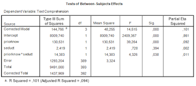
Let us get back to some of the SPSS output we considered in the previous post to get the ingredients we need for sample size planning. First, the ANOVA table.

Table 1. ANOVA source table

We are interested in estimating and optimizing the precision of an interaction contrast estimate. The first things we need are an expression of the error variance needed to calculate the standard error of the estimate and the degrees of freedom that were used in estimating the error variance. In general, the error variance needed is the same error variance you would use in performing an F-test for the specific effect, in this case the interaction effect.

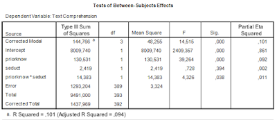
Thus, we note the error variance used to test the interaction effect, i.e. mean square error, and the degrees of freedom. The value of mean square error is 3.324, and the degrees of freedom are 389. Note that this value is the total sample sizes minus the number of conditions (393 – 4 = 389), or, equivalently, the total sample sizes minus the degrees of freedom of the intercept, the main effects, and the interaction (393 – (1 + 1 + 1 + 1) = 389). I will call these degrees of freedom the error degrees of freedom, df_e.

MOE can be obtained by multiplying a critical t-value with the same degrees of freedom as the error degrees of freedom with the standard error of the estimate.

The standard error of the contrast estimate is

$\hat{\sigma_\psi}= \sqrt{\sum{c_i^2MS_e/n_i}},$

where $c_i$ is the contrast weight for the i-th condition mean, and $n_i$ the number of observations (in our example participants) in treatment condition i. Note that $MS_e / n_i$ is the variance of treatment mean i, the square root of which gives the familiar standard error of the mean.

The contrast weights we used to estimate the 2 x 2 interaction were {-1, 1, 1, -1}. So, the expression for MOE becomes

$MOE = t_{.975}(df_e)\sqrt{\sum{c_i^2MS_e/n_i}}=t_{.975}(df_e)\sqrt{4MS_e/n_i} = 2t_{.975}(df_e)\sqrt{MS_e/n_i}.$

Thus, suppose we have the independent 2×2 factorial design, $n_i = 100$ , and the true value of Mean Square Error is 3.324, then MOE for the contrast estimate equals

$MOE = 2*t_{.975}(396)*\sqrt{3.324/100} = 0.7071$

.
Note that this is the value of MOE we obtain on average in repeated replications with new samples, if we use sample sizes of 100 (total number of participants is 400) and if the true value of the error variance is 3.324. The value is close to the value we obtained in the previous post (MOE = 0.72) because the sample sizes were very close to 100 per group.

Now, we found the original confidence interval too wide, and we have just seen how 100 participants per group does not really help. MOE is only slightly smaller than our originally obtained MOE. We need to set a target MOE and then figure out how many participants we need to get that target MOE.

Intermezzo: Rules of thumb for target MOE

(Here are some updated rules of thumb: https://the-small-s-scientist.blogspot.com/2018/11/contrast-tutorial.html)

In the absence of theoretical or practical considerations about the precision we want, we may want to use rules of thumb. My (very first proposal for) rules of thumb are based on the default interpretations of Cohen’s d. Considering the absolute values of d ≤ .10 to be negligible d = .20 small, d = .50 medium and d = .80 large. (I really do not like rules-of-thumb, because using them is a sign that you are not thinking).

Now, suppose that we interpret the confidence interval as a range of plausible values for the true value of the effect size. It is not at all clear to me what such a supposition entails, but let’s simply take it for granted right now (please don’t). Then, I think it is reasonable to say that being able to distinguish between small and negligible effects sizes is relatively precise. Thus a MOE of .05 (pooled) standard deviations can be considered precise because (on average) the 95% CI for the small effect sizes is [.15, .25], assuming we know the value of the standard deviation, so negligible effects will not be deemed plausible values on average, since effect sizes smaller than .10 are outside the interval.

By essentially the same reasoning. if we cannot distinguish between large and negligible effects, we are not estimating things very precisely. Therefore, a MOE of .80 standard deviations can be considered to be not very precise. On average, the CI for an existing large effect, will be [0, 1.60], so it includes both negligible and very large effects as plausible values.

For medium (does it make sense to speak of medium precision?) precision I would like to suggest .20-.25 standard deviations. On average, with this value for MOE, if there is a medium effect, small effects and large effects are relatively implausible. In the case of small effects, medium precision entails that on average both effects in the opposite direction and medium effects are among the plausible values.

Of course, I am interpreting the d-values as strict boundaries, but the scale is not categorical, but continuous. So instead of small, large effect sizes, it’s better to speak of smallish and largish effect sizes. And as soon as I find a variant for medium effects sizes I will also include that term in the list.

Note: sample size planning may indicate that precision of MOE = .20-.25 standard deviations is unattainable. In that case, we will simply have to accept that our precision does not lead to confident conclusions about the population effect size. (Once I showed one of my colleagues my precision app, during which he said: “that amount of precision requires a very large sample. I do not like your ideas about sample size planning”).

(By the way, I am also considering rules-of-thumb for target MOE that include assurance. Something like: high precision is when repeated experiments have a high probability of distinguishing small and negligible effects; in that case the average MOE will be smaller than .05).

Planning for precision

Let’s plan for a precision of 0.25 standard deviation. In our case, that standard deviation is the pooled standard deviation: the square root of Mean Square Error. The (estimated) value of Mean Square Error is 3.324 (see Table 1), so our value for the standard deviation is 1.8232. Our target MOE is, therefore, 0.4558.

Let’s make things very clear. Here we are planning for a target MOE based on an estimate of the pooled standard deviation (and on assumptions about the population distribution). In order for our planning to be of practical value, we need some reassurance that that estimate is trustworthy. One way of doing that is to consider the CI for the standard deviation. I will not discuss that topic, and simply give you a CI: [2.90, 3.86].

Take a look at the expression for MOE.

$MOE = 2*t_{.975}(df_e)\sqrt{(MS_w / n_i)},$

where $df_e = 4(n_i - 1)$ , since we are considering the 2×2 design.

Since our target MOE equals .4588, our goal becomes to solve the following equation for $n_i$ , since we want the sample size:

$0.4558 = 2*t_{.975}(4(n_i - 1)\sqrt{(MS_w / n_i)},$

However, because $n_i$ determines both the standard error and the degrees of freedom (and thereby the critical value of t), the equation may be a little hard to solve. So, I will create a function in R that enables me to quite easily get the required sample size. (It is relatively easy to create a more general function (see the Precision App), but here I will give an example tailored to the specific situation at hand).

First we create a function to calculate MOE:

MOE = function(n) {
  MOE = 2*qt(.975, 4*(n - 1))*sqrt(3.324/n)
}

Next, we will define a loss function and use R’s built-in optimize function to determine the sample size. Note that the loss-function calculates the squared difference between MOE based on a sample size n and our target MOE. The optimize function minimizes that squared difference in terms of sample size n (starting with n = 100 and stopping at n = 1000).

loss <- function(n) {
  (MOE(n) - 0.4558)^2
}

optimize(loss, c(100, 1000))

## $minimum
## [1] 246.4563
## 
## $objective
## [1] 8.591375e-18

Thus, according to the optimize function we need 247 participants (per group; total N = 988), to get an expected MOE equal to our target MOE. The expected MOE equals 0.4553, which you can confirm by using the MOE function we made above.

Planning with assurance

Although expected MOE is close to our target MOE, there is a probability 50% that the obtained MOE will be larger than our target MOE. In other words, repeated sampling will lead to obtained MOEs larger than what we want. That is to say, we have 50% assurance that our obtained MOE will be at least as small as our target MOE.

Planning with assurance means that we aim for a certain specified assurance that our obtained MOE will not exceed our target MOE. For instance, we may want to have 80% assurance that our obtained MOE will not exceed our target MOE.

Basically, what we need to do is take the sampling distribution of the estimate of Mean Square Error into account. We use the following formula (see also my post introducing the Precision App for the general formulae: https://the-small-s-scientist.blogspot.nl/2017/04/planning-for-precision.html).

$MOE_{\gamma} = 2*t_{.975}(df)*\sqrt{MS_w/n_i*\chi^2_{\gamma}(df)/df},$

where $gamma$ is the assurance expressed in a probability between 0 and 1.

Let’s do it in R. Again, the function that calculates assurance MOE is tailored for the specific situation, but it is relatively easy to formulate these functions in a generally applicable way,

MOE.gamma = function(n) {
  df = 4*(n-1)
  MOE = 2*qt(.975, df)*sqrt(3.324/n*qchisq(.80, df)/df)
}
loss <- function(n) {
  (MOE.gamma(n) - 0.4558)^2
}

optimize(loss, c(100, 1000))

## $minimum
## [1] 255.576
## 
## $objective
## [1] 2.900716e-18

Thus, according to the results, we need 256 persons per group (N = 1024 in total) to have a 80% probability of obtaining a MOE not larger than our target MOE. In that case, our expected MOE will be 0.4472.

July 19, 2017October 22, 2019

Planning for Precision: A confidence interval for the contrast estimate

In a previous post, which can be found here, I described how the relative error variance of a treatment mean can be obtained by combining variance components. I concluded that post by mentioning how this relative error variance for the treatment mean can be used to obtain the variance of a contrast estimate. In this post, I will discuss a little more how this latter variance can be used to obtain a confidence interval for the contrast estimate, but we take a few steps back and consider a relatively simple study.

The plan of this post is as follows. We will have a look at the analysis of a factorial design and focus on estimating an interaction effect. We will consider both the NHST approach and an estimation approach. We will use both ‘hand calculations’ and SPSS.

An important didactic aspect of this post is to show the connection between the ANOVA source table and estimates of the standard error of a contrast estimate. Understanding that connections helps in understanding one of my planned posts on how obtaining these estimates work in the case of mixed model ANOVA. See the final section of this post.

The data we will be analyzing are made up. They were specifically designed for an exam in one of the undergraduate courses I teach. The story behind the data is as follows.

Description of the study

A researcher investigates the extent to which the presence of seductive details in a text influences text comprehension and motivation to read the text. Seductive details are pieces of information in a text that are included to make the text more interesting (for instance by supplying fun-facts about the topic of the text) in order to increase the motivation of the reader to read on in the text. These details are not part of the main points in the text. The motivation to read on may lead to increased understanding of the main points in the text. However, readers with much prior knowledge about the text topic may not profit as much as readers with little prior knowledge with respect to their understanding of the text, simply because their prior knowledge enables them to comprehend the text to an acceptable degree even without the presence of seductive details.

The experiment has two independent factors, the readers’ prior knowledge (1 = Little, 2 = Much) and the presence of seductive details (1 = Absent, 2 = Present) and two dependent variables, Text comprehension and Motivation. The experiment has a between participants design (i.e. participant nested within condition).

The research question is how much the effect of seductive details differs between readers with much and readers with little prior knowledge. This means that we are interested in estimating the interaction effect of presence of seductive details and prior knowledge on text comprehension.

The NHST approach

In order to appreciate the different analytical focus between traditional NHST (as practiced) and an estimation approach, we will first take a look at the NHST approach to the analysis. It may be expected that researchers using that approach perform an ANOVA ritual as a means of answering the research question. Their focus will be on the statistical significance of the interaction effect, and if that interaction is significant the effect of seductive details will be investigated separately for participants with little and participants with much prior knowledge. The latter analysis focuses on whether these simple effects are significant or not. If the interaction effect is not significant, it will be concluded that there is no interaction effect. Of course, besides the interaction effect, the researcher performing the ANOVA ritual will also report the significance of the main effects and will conclude that main effects exist or not exist depending on whether they are significant or not. The more sophisticated version of NHST will also include an effect size estimate (if the corresponding significance test is significant) that is interpreted using rules of thumb.

The two way ANOVA output (including partial eta squared) is as follows.

Table 1. Output of traditional two-way ANOVA

The results of the analysis will probably be reported as follows.

There was a significant main effect of prior knowledge (F(1, 393) = 39.26, p < .001, partial η² = .09). Participants with much prior knowledge had a higher mean text comprehension score than the participants with little prior knowledge. There was no effect of the presence of seductive details (F < 1). The interaction effect was significant (F(1, 393) = 4.33, p < .05, partial η²= .01).

Because of the significant interaction effect, simple effects analyses were performed to further investigate the interaction. These results show a significant effect of the presence of seductive details for the participants with little knowledge (p < .05), with a higher mean score in the condition with seductive details, but for the participants with much prior knowledge no effect of seductive details was found (p = .38), which explains the interaction. (Note: with a Bonferroni correction for the two simple effects analyses the p-values are p = .08 and p = .74; this will be interpreted as that neither readers with little knowledge nor with much knowledge benefit from the presence of seductive details).

The conclusion from the traditional analysis is that the effect of seductive details differs between readers with little and readers with much prior knowledge. The presence of seductive details only has an effect on the comprehension scores of readers with little prior knowledge of the text topic, in the presence of seductive details text comprehension is higher than in the absence of seductive details. Readers with much prior knowledge do not benefit from the presence of seductive details in a text.

Comment on the NHST analysis

The first thing to note is that the NHST conclusion does not really answer the research question. Whereas the research question ask how much the effects differ, the answer to the research question is that a difference exists. This answer is further specified as that there exists an effect in the little knowledge group, but that there is no effect in the much knowledge group.

The second thing to note is that although there is a simple research questions, the report of the results includes five significance tests, while none of them actually address the research question. (Remember it is an how-much question and not a whether-question, the significance tests do not give useful information about the how-much question).

The third thing to notice is that although effect sizes estimates are included (for the significant effects only) they are not interpreted while drawing conclusions. Sometimes you will encounter such interpretations, but usually they have no impact on the answer to the research question. That is, the researcher may include in the report that there is a small interaction effect (using rules-of-thumb for the interpretation of partial eta-squared; .01 = small; .06 = medium, .14 = large), but the smallness of the interaction effect does not play a role in the conclusion (which simply reformulates the (non)significance of the results without mentioning numbers; i.e. that the effect exists (or was found) in one group but not in the other).

As an aside, the null-hypothesis test for the effect of prior knowledge i.e. that the mean comprehension score of readers with little knowledge are equal to the mean comprehension score of readers with much prior knowledge about the text topic seems to me an excellent example of a null-hypothesis that is so implausible that rejecting it is not really informative. Even if used as some sort of manipulation check the real question is the extent to which the groups differ and not whether the difference is exactly zero. That is to say, not every non-zero difference is as reassuring as every other non-zero difference: there should be an amount of difference between the groups below which the group performances can be considered to be practically the same. If a significance tests is used at all, the null-hypothesis should specify that minimum amount of difference.

Estimating the interaction effect

We will now work towards estimating the interaction effect. We will do that in a number of steps. First, we will estimate the value of the contrasts on the basis of the estimated marginal means provided by the two-way ANOVA and show how the confidence interval of that estimate can be obtained. Second, we will use SPSS to obtain the contrast estimate.

Table 2 contains the descriptives and samples sizes for the groups and the estimated marginal means are presented in Table 3.

Table 2. Descriptive Statistics

Table 3. Estimated Marginal Means

Let’s spend a little time exploring the contents of Table 3. The estimated means speak for themselves, hopefully. These are simply estimates of the population means.

The standard errors following the means are used to calculate confidence intervals for the population means. The standard error is based on an estimate of the common population variance (the ANOVA model assumes homogeneity of variance and normally distributed residuals). That estimate of the common variance can be found in Table 1: it is the Mean Square Error. Its estimated value is 3.32, based on 389 degrees of freedom.

The standard errors of the means in Table 3 are simply the square root of the Mean Square Error dvided by the sample size. E.g. the standard error of the mean text comprehension in the group with little knowledge and seductive details absent equals √(3.32/94) = .1879.

The Margin of Error needed to obtain the confidence interval is the critical t-value with 389 degrees of freedom (the df of the estimate of Mean Square Error) multiplied by the standard error of the mean. E.g. the MOE of the first mean is t_.975(389)*.1879 = 1.966*.1879 = 0.3694.

The 95%-confidence interval for the first mean is therefore 3.67 +/- 0.3694 = [3.30, 4.04].

Contrast estimate

We want to know the extent to which the effect of seductive details differs between readers with little and much prior knowledge. This means that we want to know the difference between the differences. Thus, the difference between the means of the Present (P) and Absent (A) of readers with Much (M) knowledge is subtracted from the difference between the means of the readers with Little (L) knowledge: (M_L+P – M_L+A) – (M_M+P – M_M+A) = M_L+P – M_L+A – M_M+P + M_M+A = 4.210 – 3.670 – 4.980 + 5.206 = 0.766.

Our point estimate of the difference between the effect of seductive details for little knowledge readers and for much knowledge is that the effect is 0.77 points larger in the group with little knowledge.

For the interval estimate we need the estimated standard error of the contrast estimate and a critical value for the central t-statistic. To begin with the latter: the degrees of freedom are the degrees of freedom used to estimate Mean Square Error (df = 389; see Table 1).

The standard error of the contrasts estimate can be obtained by using the variance sum law. That is, the variance of the sum of two variables is the sum of their variances plus twice the covariance. And the variance of the difference between two variables is the sum of the variances minus twice the covariance. In the independent design, all the covariances between the means are zero, so the variance of the interaction contrast is simply the sum of the variances over the means. The standard error is the square root of this figure. Thus, var(interaction contrast) = 0.188² + 0.182² + 0.185² + 0.181² = 0.1354, and the standard error of the contrast is the square root of 0.1354 = .3680.

Note that the we have squared the standard errors of the mean. These squared standard error are the same as the relative error variances of the means. (Actually, in a participant nested under treatment condition (a between-subject design) the relative error variance of the mean equals the absolute error variance). More information about the error variance of the mean can be found here: https://the-small-s-scientist.blogspot.nl/2017/05/PFP-variance-components.html.

The Margin of Error of the contrast estimate is therefore t_.975(389)*.3680 = 1.966*.3680 = 0.7235. The 95% confidence interval for the contrast estimate is [0.04, 1.49].

Thus, the answer to the research question is that the estimated difference in effect of seductive details between readers with little prior knowledge and readers with much prior knowledge about the text topic equals .77, 95% CI [.04, 1.49]. The 95% confidence interval shows that the estimate is very imprecise, since the limits of the interval are .04, which suggests that the effect of seductive details is essentially similar for the different groups of readers, and 1.49, which shows that the effect of seductive details may be much larger for little knowledge readers than for much knowledge readers.

Analysis with SPSS

I think it is easiest to obtain the contrast estimate by modeling the data with one-way ANOVA by including a factor I’ve called ‘independent’. (Note: In this simple case, the parameter estimates output of the independent factorial ANOVA also gives the interaction contrast (including the 95% confidence interval), so there is no actual need to specify contrasts, but I like to have the flexibility of being able to get an estimate that directly expresses what I want to know). This factor has 4 levels: one for each of the combinations of the factors prior knowledge and presence of seductive details: Little-Absent (LA), Little-Present (LP), Much-Absent (MA), and Much-Present (MP).

The interaction we’re after is the difference between the mean difference between Present and Absent for participants with little knowledge (M_LP – M_LA) and the mean difference between Present and Absent in the much knowledge group (M_MP – M_MA). Thus, the estimate of the interaction (difference between differences) is (M_LP – M_LA) – (M_MP – M_MA) = M_LP – M_LA – M_MP + M_MA. This can be rewritten as 1*M_LP + -1*M_LA + -1*M_MP + 1*M_MA).

The 1’s and -1’s are of course the contrast weights we have to specify in SPSS in order to get the estimate we want. We will have to make sure that the weights correspond to the way in which the order of the means is represented internally in SPSS. That order is LA, LP, MA, MP. Thus, the contrast weights need to be specified in that order to get the estimate to express what we want in terms of the difference between differences. See the second line in the following SPSS-syntax.

UNIANOVA comprehension BY independent
/CONTRAST(independent)=SPECIAL ( -1 1 1 -1)
/METHOD=SSTYPE(3)
/INTERCEPT=INCLUDE
/EMMEANS=TABLES(independent)
/PRINT=DESCRIPTIVE
/CRITERIA=ALPHA(.05)
/DESIGN=independent.

The relevant output is presented in Table 4. Note that the results are the same as the ‘hand calculations’ described above (I find this very satisfying).

Table 4. Interaction contrast estimate

Comment on the analysis

First note that the answer to the research question has been obtained with a single analysis. The analysis gives us a point estimate of the difference between the differences and a 95% confidence interval. The analysis is to the point to the extent that it gives the quantitative information we seek.

However, although the estimate of the difference between the differences is all the quantitative information we need to answer the how-much-research question, the estimate itself obscures the pattern in the results, in the sense that the estimate itself does not tell us what may be important for theoretical or practical reasons, namely the direction of the effect. That is, a positive interaction contrast may indicate the difference between an estimated positive effect for one group and an estimated negative effect in the other group (which is actually the situation in the present example: 0.54 – (-0.23) = 0.77) in the other group).

Of course, we could argue that if you want to know the extent to which the size and direction differ between the groups, then that should be reflected in your research question, for instance, by asking about and estimating the simple effects themselves in stead of focusing on the size of the difference alone, as we have done here.

On the other hand, we could argue that no result of a statistical analysis should be interpreted in isolation. Thus, there is no problem with interpreting the estimate of 0.77 while referring to the simple effects: the estimated difference between the effects is .77, 95% CI [.04, 1.49], reflecting the difference between an estimated effect of 0.54 in the little knowledge group and an estimated negative effect of -0.23 for much knowledge readers.

But, if the research question is how large is the effect of seductive details for little knowledge readers and high knowledge readers and how much do the effect differ, than that would call for three point estimates and interval estimates. Like: the estimated effect for the little knowledge group equals 0.54. 95% CI [0.03, 1.06], whereas the estimated effect for the much knowledge groups is negative -0.23, 95% CI [-0.73, 0.28]. The difference in effect is therefore 0.77, 95% CI [.04, 1.49].

In all cases, of course, the intervals are so wide that no firm conclusions can be drawn. Consistent with the point estimates are negligibly small positive effects to large positive effects of seductive details for the little knowledge group, small positive effects to negative effects of seductive details for the much knowledge group and an interaction effect that ranges from negligibly small to very large. In other words, the picture is not at all clear. (Interpretations of the effect sizes are based on rules of thumb for Cohen’s d. A (biased) estimate of Cohen’s d can be obtained by dividing the point estimate by the square root of Mean Square Error. An approximate confidence interval can be obtained by dividing the end-points of the non-standardized confidence intervals by the square root of Mean Square Error). Of course, we have to keep in mind that 5% of the 95% confidence intervals do not contain the true value of the parameter or contrast we are estimating.

Compare this to the firm (but unwarranted) NHST conclusion that there is a positive effect of seductive details for little knowledge readers (we don’t know whether there is a positive effect, because we can make a type I error if we reject the null) and no effect for much knowledge readers. (Yes, I know that the NHST thought-police forbids interpreting non-significant results as “no effect”, but we are talking about NHST as practiced and empirical research shows that researchers interpret non-significance as no effect).

In any case, the wide confidence intervals show that we could do some work for a replication study in terms of optimizing the precision of our estimates. In a next post, I will show you how we can use our estimate of precision for planning that replication study.

Summary of the procedure

In (one of the next) posts, I will show that in the case of mixed models ANOVA’s we frequently need to estimate the degrees of freedom in order to be able to obtain MOE for a contrast. But the basic logic remains the same as what we have done in estimating the confidence interval for the interaction contrast. Please keep in mind the following.

Looking at the ANOVA source table and the traditional ANOVA approach we notice that the interaction effect is tested against Mean Square Error: the F-ratio we use to test the null-hypothesis that both Mean Squares (the interaction MS an Mean Square Error) estimate the common error variance. The F-ratio is formed by dividing the Mean Square associated with the interaction by Mean Square Error. The probability distribution of that ratio is an F-distribution with 1 (numerator) and 389 (denominator) degrees of freedom.

Mean Square Error is also used to obtain the estimated standard error for the interaction contrast estimate. In the calculation of MOE, the critical value of t was determined on the basis of the degrees of freedom of Mean Square Error.

This is the case in general: the standard error of a contrast is based on the Mean Square Error that is also used to test the corresponding Effect (main or interaction) in an F-test. In a simple two-way ANOVA the same Mean Square Error is used to test all the effects (main an interaction), but that is not generally the case for more complex designs. Also, the degrees of freedom used to obtain a critical t-value for the calculation of MOE are the degrees of freedom of the Mean Square Error used to test an effect.

In the case of a mixed model ANOVA, it is often the case that there is no Mean Square Error available to directly test an effect. The consequence of this is that we work with linear combinations of Mean Squares to obtain a suitable Mean Square Error for an effect and that we need to estimate the degrees of freedom. But the general logic is the same: the Mean Square Error that is obtained by a linear combination of Mean Squares is also used to obtain the standard error for the contrast estimate and the estimated degrees of freedom are the degrees of freedom used to obtain a critical value for t in the calculation of the Margin of Error.

I will try to write about all of that soon.

May 4, 2017October 22, 2019

Planning for Precision: Introduction to variance components

Both theory underlying the Precision application and the use of the app in practice rely for a large part on specifying variance components. In this post, I will give you some more details about what these components are, and how they relate to the analysis of variance model underlying the app.

What is variance?

Let’s start with a relatively simple conceptual explanation of variance. The key ideas are expected value and error. Suppose you randomly select a single score from a population of possible values. Let’s suppose furthermore that the population of values can be described with a normal distribution. There is actually no need to suppose a normal distribution, but it makes the explanation relatively easy to follow.

As you probably know, the normal distribution is centered around its mean value, which is (equal to) the parameter μ. We call this parameter the population mean.

Now, we select a single random value from the population. Let’s call this value X. Because we know something about the probability distribution of the population values, we are also in the position to specify an expected value for the score X. Let’s use the symbol E(X) for this expected value. The value of E(X) proves (and can be proven) to be equal to the parameter μ. (Conceptually, the expectation of a variable can be considered as its long run average).

Of course, the actual value obtained will in general not be equal to the expected value, at least not if we sample from continuous distributions like the normal distribution. Let’s call the difference between the value X and it’s expectation E(X) = μ. an error, deviation or residual: e = X – E(X) = X – μ.

We would like to have some indication of the extent to which X differs from its expectation, especially when E(X) is estimated on the basis of a statistical model. Thus, we would like to have something like E(X – E(X)) = E(X – μ). The variance gives us such an indication, but does so in squared units, because working with the expected error itself always leads to the value 0 E(X – μ) = E(X) – E( μ) = μ – μ = 0. (This simply says that on average the error is zero; the standard explanation is that negative and positive errors cancel out in the long run).

The variance is the expected squared deviation (mean squared error) between X and its expectation: E((X – E(X))²) = E(X – μ)²), and the symbol for the population value is σ².

Some examples of variances (remember we are talking conceptually here):
– the variance of the mean, is the expected squared deviation between a sample mean and its expectation the population mean.
– the variance of the difference between two means: the expected squared deviation between the sample difference and the population difference between two means.
– the variance of a contrast: the expected squared deviation between the sample value of the contrast and the population value of the contrast.

It’s really not that complicated, I believe.

Note: in the calculation of t-tests (and the like), or in obtaining confidence intervals, we usually work with the square root of the variance: the root mean squared error (RMSE), also known as the standard deviation (mostly used when talking about individual scores) or standard error (when talking about estimating parameter values such as the population mean or the differences between population means).

What are variance components?

In order to appreciate what the concept of a variance component entails, imagine an experiment with n_c treatment conditions in which n_p participants respond to n_i items (or stimuli) in all conditions. This is called a fully-crossed experimental design.

Now consider the variable X_cpi. a random score in condition t, of participant p responding to item i. The variance of this variable is σ²(X_cpi) = E((X_cpi – μ)²). But note that just as the single score is influenced by e.g. the actual treatment condition, the particular person or item, so too can this variance be decomposed into components reflecting the influence of these factors. Crucially, the total variance σ²(X_cpi) can be considered as the sum of independent variance components, each reflecting the influence of some factor or interaction of factors.

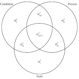
The following figure represents the components of the total variance in the fully crossed design (as you can see the participants are now promoted to actual persons…)

The symbols used in this figure represent the following. Θ² is used to indicate that a component is considered to be a so-called fixed variance component (the details of which are beyond the scope of this post), and the symbol σ² is used to indicate components associated with random effects. (The ANOVA model contains a mixture of fixed and random effects, that’s why we call such models mixed effects models or mixed model ANOVAs). Components with a single subscript represent variances associated with main effects, components with two subscripts two-way interactions, and the only component with three subscripts represents a three-way-interaction confounded with error.

Let’s consider one of these variance components (you can also refer to them simply as variances) to see in more detail how they can be interpreted. Take σ²(p), the person-variance. Note that this is an alternative symbol for the variance, in the figure, the p is in the subscript in stead of between brackets (I am sorry for the inconvenience of switching symbols, but I do not want to rely too much on mathjax ($sigma^2_p = sigma^2(p)$) and I do not want to change the symbols in the figure).

The variance σ²(p) is the expected squared deviation of the score of an idealized randomly selected person and the expectation of this score, the population mean. This score is the person score averaged of the conditions of the experiment and all of the items that could have been selected for the experiment. (This conceptualization is from Generalizability Theory; the Venn-diagram representation as well), the person score is also called the universe score of the person).

The component represents E((μ_p – μ)²), the expected squared person effect. Likewise, the variance associated with items σ²(i) is the expected squared item effect, and σ²(cp), is the expected squared interaction effect of condition and person.

The figure indicates that the total variance is (modeled as) the sum of seven independent variance components. The Precision app asks you to supply the values for six of these components (the components associated with the random effects), and now I hope it is a little clearer why these components are also referred to as expected squared effects.

Relative error variance of a treatment mean

The basic goal of contrast analysis is to compare a mean (or more) relative to one (or more) other treatment means. That is, we are interested in the relative position of a mean compared to the rest. Due to sampling error our estimate of the relative position of a mean differs from the ‘true’ relative position. The relative error variance of a treatment mean is the expected squared deviation between the obtained relative position and the expected relative position.

Let’s consider the Venn-diagram above again. In particular, take a look at the condition-circle and the components contained in it. A total of four variance components are included in the circle. The component Θ²(c), is the component associated with the treatment effect (μ_c – μ). All the other components contained in the circle contribute to the relative error variance. Thus, the interaction of treatment and participant, the interaction of treatment and stimulus, and the error contribute to the deviation between the true effect (relative position) and the estimated effect. Or, in other words, the relative error variance of the treatment mean consists of the three variance components associated with the treatment by participant interaction, the treatment by stimulus interaction, and error.

But these components specify the variance in terms of individual measurements, whereas the treatment mean is obtained on the basis of averaging over the n_p*n_i measurements we have in the corresponding treatment condition. So let’s see how we can take into account the number of measurements.

Unfortunately, things get a little complicated to explain, but I’ll have a go nonetheless. The explanation takes two steps: 1) We consider how to specify expected mean squares in terms of the components contained in the condition-circle 2) We’ll see how to get from the formulation of the expected mean square to the formulation of the relative error variance of a treatment mean.

Obtaining an expected mean square

I will use the term Mean Square (MS) to refer to a variance estimate. For instance, MS_T is an estimate of the variance associated with the treatment condition. The expected MS (EMS) is the average value of these estimates.

We can use the Venn-diagram to obtain an EMS for the treatment factor and all the other factors in the design, but we will focus on the EMS associated with treatment. However, we cannot use the variance components directly, because the mixed ANOVA model I have been using for the application contains sum-to-zero restrictions on the treatment effects and the two-way interaction-effects of treatment and participant and treatment and stimulus (item). The consequence of this is that we will have to multiply the variance components associated with the treatment-by-participant and treatment-by-stimulus with a constant equal to n_c / (n_c – 1), where n_c is the number of conditions.(This is the hard part to explain, but I didn’t really explain it, but simply stated it).

The second step of obtaining the EMS is to multiply the components with the number of participants and items, as follows. Multiply the component by the sample size if and only if the subscript of the component does not contain a reference to the particular sample size. That is, for instance, multiply a component by the number of participants n_p, if and only if the subscript of the component does not contain a subscript associated with participants.

This leads to the following:

E(MST) = n_pn_iΘ²(T) + n_i(n_c / (n_c – 1))σ²(cp) + n_p(n_c / (n_c – 1))σ²(ci) + σ²(cpi, e).

Obtaining the relative error variance of the treatment mean

Notice that n_i(n_c / (n_c – 1))σ²(cp) + n_p(n_c / (n_c – 1))σ²(ci) + σ²(cpi, e) contains the components associated with the relative error variance. Because the treatment mean is based on n_p*n_i scores, to obtain the relative error variance for the treatment mean, we divide by n_p*n_i to obtain.

Relative error variance of the treatment mean = (n_c / (n_c – 1))σ²(cp) / n_p + (n_c / (n_c – 1))σ²(ci) / n_i+ σ²(cpi, e) / (n_pn_i).

As an aside, in the post describing the app, I have used the symbols σ²(αβ) to refer to n_c / (n_c – 1))σ²(cp), and σ²(αγ) to refer to (n_c / (n_c – 1))σ²(ci).

Comparing means: the error variance of a contrast

From the relative error variance of a treatment mean, we can get to the variance of a contrast, simply by multiplying the relative error variance by the sum of the squared contrast weights. For instance, if we want to compare two treatment means we can do so by estimating the contrast ψ = 1*μ₁ + (-1)*μ₂, where the values 1 and (-1) are the contrast weights. The sum of the squared contrast weights equals 2, the error variance of the contrast is therefore 2*(n_c / (n_c – 1))σ²(cp) / n_p + (n_c / (n_c – 1))σ²(ci) / n_i+ σ²(cpi, e) / (n_pn_i).

Note that the latter gives us the expected squared deviation between the estimated contrast value and the true contrast value (see also the explanation of the concept of variance above).

It should be noted that for the calculation of a 95% confidence interval for the contrast estimate (or for the Margin of Error; the half-width of the confidence interval) we make use of the square root of the error variance of the contrast. This square root is the standard error of the contrast estimate. The calculation of MOE also requires a value for the degrees of freedom. I will write about forming a confidence interval for a contrast estimate in one of the next posts.

May 3, 2017October 22, 2019

Planning for Precision: simulation results for four designs with four conditions

This is the third post about the Planning for Precision app (in the future I’ll explain the difference between Planning for Precision and Precision for Planning). Some background information about the application can be found here: http://the-small-s-scientist.blogspot.com/2017/04/planning-for-precision.html.

In this post, I want to present the simulation results for 4 designs with 4 conditions. The designs are: the counter balanced design (see previous post), the fully-crossed design, the stimulus-within-condition design, and the stimulus-and-participant-within-condition design (the both-within-condition design). I have not included the participants-within-condition design, because this is simply the mirror-image (so to say) of the stimulus-within-condition design.

In one of my next posts, I will describe some more background information about planning for precision, but some of the basics are as follows. We have a design with 4 treatment conditions, and what we want do is to estimate differences between these condition means by using contrasts. For instance, we may be interested in the (amount of) difference between the first mean, maybe because it is a control-condition with the average of the other three conditions: μ₁ – (μ₂ + μ₃ + μ₄)/3 = 1*μ₁ – 1/3*μ₂ -1/3*μ₃ – 1/3*μ₄. The values {1, -1/3, -1/3, -1/3} are the contrast weights, and for the result we use the term ψ.

The value of ψ is estimated on the basis of estimates of the population means, that is, the sample means or condition means. Due to sampling error, the contrast estimate varies from sample to sample and the amount of sampling error can be expressed by means of a confidence interval. Conceptually, the confidence interval expresses the precision of the estimate: the wider the confidence interval, the less precise the estimate is.

The Margin of Error (MOE) of an estimate is the half-width of the confidence interval, so the confidence interval is the estimate plus or minus MOE. We will take MOE as an expression of the precision of the estimate (the less the value of MOE the more precise the estimate). Now, if you want to estimate an effect size, more precision (lower value of MOE; less wide confidence interval) is better than less precision (higher value of MOE; wider confidence interval). The app let’s you specify the design and the contrast weights and helps you find the minimum required sample sizes (for participants and stimuli) for a given target MOE. (You can also play with the designs to see which design gives you smallest expected MOE).

Crucially, if you plan for precision, you also want to have some assurance that the MOE you are likely to obtain in you actual experiment will not be larger than you target MOE. Compare this with power: 80% power means that the probability that you will reject the null-hypothesis is 80%. Likewise, assurance MOE of 80% means that there is an 80% probability that your obtained MOE will be no larger than assurance MOE.

The simulations (with N = 10000 replications) estimate Expected MOE as well as Assurance MOE for assurances of .80, .90, .95, and .99, for 4 designs with 4 treatment conditions, with a total number of 48 participants and 24 stimuli (items). The MOEs are given for three standard constrasts: 1) the difference between the first mean and the mean of the other three, with weights {1, -1/3, -1/3, -1/3}; 2) the difference between the second mean and the mean of conditions three and four, with weights {0, 1, -1/2, -1/2}; 3) the difference between the third and fourth condition means, with weights {0, 0, 1, -1}.

I will present the results in separate tables for the 4 designs considered and include percentage difference between expected values of assurance MOE and the estimated values estimated values.

The fully crossed design

The results are in the following table.

The percentage difference between the expected quantiles (= assurance MOEs for given insurance; i.e. q.80 is expected or estimated 80% Assurance MOE) and the estimated quantiles are: .80: 0.11%; .90: 0.05%; .95: -0.14%; 99: -0.05%.

The counter balanced design

The results are presented in the following table.

The percentage difference between the expected quantiles and the estimated quantiles are: .80: 0.03%; .90: 0.13%; .95: 0.09%, .99: -0.23%.

The stimulus-within-condition design

The following table contains the details.

The percentage difference between the expected quantiles and the estimated quantiles are: .80: -0.11%; .90: -0.33%; .95: -0.55%, .99: -0.70%.

Both-participant-and-stimulus-within-condition design

Here is the table.

And the percentage differences are: .80: -0.34%; .90: -0.59%; .95: -0.82%; .99: -1.06%.

Conclusion

The results show that the simulation results are quite consistent with the expected values based on mixed model ANOVA. We can see that the differences between expected and estimated values increase the less the number of participants and items per condition. For instance, in the both within condition design 12 participants respond to 6 stimuli in one of the four treatment conditions. The fact that even with these small samples sizes the results seem to agree to an acceptable degree is (to my mind) encouraging. Note that with small samples the expected assurance MOES are slightly lower than the estimates, but the largest difference is -1.06% (see the MOE for 99% assurance).

May 1, 2017October 22, 2019

Planning for Precision: first simulation results

In this post, I want to share the results of the first simulation study to “test” my Planning for Precision app. More details about the app can be found in a previous post: here.

I have included the basic logic of the simulations (including R code) in a document that you can download: https://drive.google.com/open?id=0B4k88F8PMfAhSlNteldYRWFrQTg.

The simulation study simulates responses from a four condition counter balanced design, with p = 48 participants and q = 24 stimuli/items. Here, we will focus on expected and assurance MOE for three contrasts. The first contrast estimates the difference between the first mean and the average of the other three, the second contrast the difference between the second mean and the average of the third and fourth means, and the final contrast the difference between the means of the third and fourth contrasts.

Expected MOE is compared to the mean of the estimated MOE for each of the contrasts (based on 10000 replications). Assurance MOE is judged for assurance of .80, .90, .95 and .99, by comparing the calculations in the app with the corresponding quantile estimates of the simulated distributions.

Results

Note that in the above table, the Expected Mean MOE is what I have called Expected MOE, and the q.80 through q.99 are quantiles of the distribution of MOE. As an example, q.80 is the quantile corresponding to assurance MOE with 80% assurance, Expected q.80 is the value of assurance MOE calculated with the theoretical approach, and Estimated q.80 is the estimated quantile based on the simulation studies.

Importantly, we can see that most of the figures agree to a satisfying degree. If we look at the relative differences, expressed in percentages for the assurance MOEs, we get 0.0325% for q.80, 0.1260% for q.90, 0.0933% for q.95, and -0.2324% for q.99.

Conclusion

The first simulation results seem promising. But I still have a lot of work to do for the rest of the designs.

April 29, 2017June 9, 2021

Planning for precision with samples of participants and items

Many experiments involve the (quasi-)random selection of both participants and items. Westfall et al. (2014) provide a Shiny-app for power-calculations for five different experimental designs with selections of participants and items. Here I want to present my own Shiny-app for planning for precision of contrast estimates (for the comparison of up to four groups) in these experimental designs. The app can be found here: https://gmulder.shinyapps.io/precision/

(Note: I have taken the code of Westfall’s app and added code or modified existing code to get precision estimates in stead of power; so, without Westfall’s app, my own modified version would never have existed).

The plan for this post is as follows. I will present the general theoretical background (mixed model ANOVA combined with ideas from Generalizability Theory) by considering comparing three groups in a counter balanced design.
Note 1: This post uses mathjax, so it’s probably unreadable on mobile devices. Note: a (tidied up) version (pdf) of this post can be downloaded here: download the pdf
Note 2: For simulation studies testing the procedure go here: https://the-small-s-scientist.blogspot.nl/2017/05/planning-for-precision-simulation.html
Note 3: I use the terms stimulus and item interchangeably; have to correct this to make things more readable and comparable to Westfall et al. (2014).
Note 4: If you do not like the technical details you can skip to an illustration of the app at the end of the post.

The general idea

The focus of planning for precision is to try to minimize the half-width of a 95%-confidence interval for a comparison of means (in our case). Following Cumming’s (2012) terminology I will call this half-width the Margin of Error (MOE). The actual purpose of the app is to find required sample sizes for participants and items that have a high probability (‘assurance’) of obtaining a MOE of some pre-specified value.

Expected MOE for a contrast

For a contrast estimate $\hat{\psi}$ we have the following expression for the expected MOE.

$E(MOE) = t_{.975}(df)*\sigma_{\hat{\psi}},$

where $\sigma_{\hat{\psi}}$ is the standard error of the contrast estimate. Of course, both the standard error and the df are functions of the sample sizes.

For the standard error of a contrast with contrast weights $c_i$ through $c_a$ , where a is the number of treatment conditions, we use the following general expression.

$\sigma_{\hat{\psi}} = \sqrt{\sum c^2_i \frac{\sigma^2_w}{n}},$

where n is the per treatment sample size (i.e. the number of participants per treatment condition times the number of items per treatment condition) and $\sigma^2_w$ the within treatment variance (we assume homogeneity of variance).

For a simple example take an independent samples design with n = 20 participants responding to 1 item in one of two possible treatment conditions (this is basically the set up for the independent t-test). Suppose we have contrast weights $c_1 = 1$ and $c_2 = -1$ , and $\sigma^2_w = 20$ , the standard error for this contrast equals $\sigma_{\hat{\psi}} = \sqrt{\sum c^2_i\frac{\sigma^2_w}{n}} = \sqrt{2*20/20} = \sqrt{2}$ . (Note that this is simply the standard error of the difference between two means as used in the independent samples t-test).

In this simple example, df is the total sample size (N = n*a) minus the number of treatment conditions (a), thus $df = N - a = 38$ . The expected MOE for this design is therefore, $E(MOE) = t_{.975}(38)*\sqrt{2} = 2.0244*1.4142 = 2.8629$ . Note that using these figures entails that 95% of the contrast estimates will take values between the true contrast value plus and minus the expected MOE: $\psi \pm 2.8629$ .

For the three groups case, and contrast weights { $1, -1/2, -1/2$ }, the same sample sizes and within treatment variance gives $E(MOE) = t_{.975}(57)*\sqrt{1.5*\frac{20}{20}} = 2.4525$ .

(If you like, I’ve written a little document with derivation of the variance of selected contrast estimates in the fully crossed design for the comparison of two and three group means. That document can be found here: https://drive.google.com/open?id=0B4k88F8PMfAhaEw2blBveE96VlU)

The focus of planning for precision is to try to find sample sizes that minimize expected MOE to a certain target MOE. The app uses an optimization function that minimizes the squared difference between expected MOE and target MOE to find the optimal (minimal) sample sizes required.

Planning with assurance

If the expected MOE is equal to target MOE, the sample estimate of MOE will be larger than your target MOE in 50% of replication experiments. This is why we plan with assurance (terminology from Cumming, 2012). For instance, we may want to have a 95% probability (95% assurance) that the estimated MOE will not exceed our target MOE.

In order to plan with assurance, we need (an approximation of) the sampling distribution of MOE. In the ANOVA approach that underlies the app, this boils down to the distribution of estimates of $\sigma^2_w$ :

$MS_w \sim \sigma^2_w*\chi^2(df)/df,$

thus

$\hat{MOE} \sim t_{.975}(df)\sqrt{\frac{1}{n}\sum{c_i^2}\sigma^2_w*\chi^2(df)/df}.$

In terms of the two-groups independent samples design above: the expected MOE equals 2.8629. But, with df = 38, there is an 80% probability (assurance) that the estimated MOE will be no larger than:

$\hat{MOE}_{.80} = 2.0244 * \sqrt{1/20*2*20*45.07628/38} = 3.1181.$

Note that the 45.07628 is the quantile $q_{.80}$ in the chi-squared (df = 38) distribution. That is $P(\chi^2(38) \leq 45.07628) = .80$ .

The app let’s you specify a target MOE and a value for the desired assurance ( $\gamma$ ) and will find the combination of number of participants and items that will give an estimated MOE no larger than target MOE in $\gamma$ % of the replication experiments.

The mixed model ANOVA approach

Basically, what we need to plan for precision is to able to specify $\sigma^2_w$ and the degrees of freedom. We will specify $\sigma^2_w$ as a function of variance components and use the Satterthwaite procedure to approximate the degrees of freedom by means of a linear combination of expected mean squares. I will illustrate the approach with a three-treatment conditions counterbalanced design.

A description of the design

Suppose we are interested in estimating the differences between three group means. We formulate two contrasts: one contrast estimates the mean difference between the first group and the average of the means of the second and third groups. The weights of the contrasts are respectively {1, -1/2, -1/2}, and {0, 1, -1}.

We are planning to use a counterbalanced design with a number of participants equal to p and a sample of items of size q. In the design we randomly assign participants to a groups, where a is the number of conditions, and randomly assign items to a lists (see Westfall et al., 2014 for more details about this design). All the groups are exposed to all lists of stimuli, but the groups are exposed to different lists in each condition. The number of group by list combinations equals $a^2$ , and the number of observations in each group by list combination equals $\frac{1}{a^2}pq$ . The condition means are estimated by combining a group by list combinations each of which composed of different participants and stimuli. The total number of observations per condition is therefore, $\frac{a}{a^2}pq = \frac{1}{a}pq$ .

The ANOVA model

The ANOVA model for this design is

$Y_{ijk} = \mu + \alpha_i + \beta_j + \gamma_k + (\alpha\beta)_{ij} + (\alpha\gamma)_{ik} + e_{ijk},$

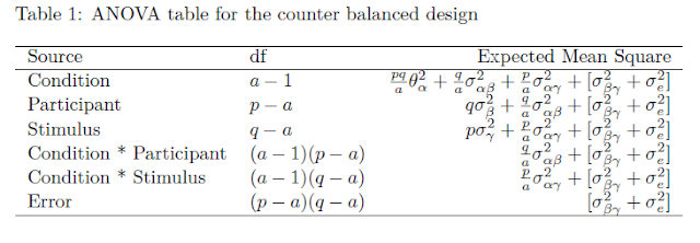
where the effect $\alpha_i$ is a constant treatment effect (it’s a fixed effect), and the other effect are random effects with zero mean and variances $\sigma^2_\beta$ (participants), $\sigma^2_\gamma$ (items), $\sigma^2_{\alpha\beta}$ (person by treatment interaction), $\sigma^2_{\alpha\gamma}$ (item by treatment interaction) and $\sigma^2_e$ (error variance confounded with the person by item interaction). Note: in Table 1 below, $\sigma^2_e$ is (for technical reasons not important for this blogpost) presented as this confounding $[\sigma^2_{\beta\gamma} + \sigma^2_e]$ .

We make use of the following restrictions (Sahai & Ageel, 2000): $\sum_{i = 1}^a = 0$ , and $\sum_{i=1}^a(\alpha\beta)_{ij} = \sum_{i=1}^a(\alpha\gamma)_{ik} = 0$ . The latter two restrictions make the interaction-effects correlated across conditions (i,e. the effects of person and treatment are correlated across condition for the same person, likewise the interaction effects of item and treatment are correlated across conditons for the same item. Interaction effects of different participants and items are uncorrelated). The covariances between the random effects $\beta_j, \gamma_i, (\alpha\beta)_{ij}, (\alpha\gamma)_{ik}, e_{ijk}$ are assumed to be zero.

Under this model (and restrictions) $E((\alpha\beta)^2) = \frac{a - 1}{a}\sigma^2_{\alpha\beta}$ , and $E((\alpha\gamma)^2) = \frac{a - 1}{a}\sigma^2_{\alpha\gamma}$ . Furthermore, the covariance of the interactions between treatment and participant or between treatment and item for the same participant or item are $-\frac{1}{a}\sigma^2_{\alpha\beta}$ for participants and $-\frac{1}{a}\sigma^2_{\alpha\gamma}$ for items.

Within treatment variance

In order to obtain an expectation for MOE, we take the expected mean squares to get an expression or the expected within treatment variance $\sigma^2_w$ . These expected means squares are presented in Table 1.

The expected within treatment variance can be found in the Treatment row in Table 1. It is comprised of all the components to the right of the component associated with the treatment effect ( $\theta^2_a$ ). Thus, $\sigma^2_w = \frac{q}{a}\sigma^2_{\alpha\beta} + \frac{p}{a}\sigma^2_{\alpha\gamma}+[\sigma^2_{\beta\gamma} + \sigma^2_e]$ . Note that the latter equals the sum of the expected mean squares of the Treatment by Participant ( $E(MS_{tp})$ ) and the Treatment by Item ( $E(MS_{ti})$ ) interactions, minus the expected mean square associated with Error ( $E(MS_e)$ ).

Degrees of freedom

The second ingredient we need in order to obtain expected MOE are the degrees of freedom that are used to estimate the within treatment variance. In the ANOVA approach the within treatment variance is estimated by a linear combination of mean squares (as described in the last sentence of the previous section. This linear combination is also used to obtain approximate degrees of freedom using the Satterthwaite procedure:

$df =\frac{(E(MS_{tp}) + E(MS_{ti}) - E(MS_e))^2}{\frac{E(MS_{tp})^2}{(a - 1)(p-a)}+\frac{E(MS_{ti})^2}{(a - 1)(q-a)}+\frac{E(MS_e)^2}{(p-a)(q-a)}}$

Expected MOE

(Note: I can’t seem to get mathjax to generate align environments or equation arrays, so the following is ugly; Note to self: next time use R-studio or Lyx to generate R-html or an equivalent format).

The expected value of MOE for the contrasts in the counter balanced design is:

$E(MOE) = t(df)*\sqrt{(\sum_{i=1}^a c^2_i)(\frac{1}{a}pq)^{-1}\sigma^2_w}$

$= t(df)*\sqrt{(\sum_{i=1}^a c^2_i)(\frac{1}{a}pq)^{-1}(\frac{q}{a}\sigma^2_{\alpha\beta} + \frac{p}{a}\sigma^2_{\alpha\gamma}+[\sigma^2_{\beta\gamma} + \sigma^2_e])}$

$=t(df)*\sqrt{(\sum_{i=1}^a c^2_i)(pq)^{-1}(q\sigma^2_{\alpha\beta} + p\sigma^2_{\alpha\gamma}+a[\sigma^2_{\beta\gamma} + \sigma^2_e])}$

$=t(df)*\sqrt{(\sum_{i=1}^a c^2_i)(\sigma^2_{\alpha\beta}/p + \sigma^2_{\alpha\gamma}/q +a[\sigma^2_{\beta\gamma} + \sigma^2_e]/pq)}$

Finally an example

Suppose we the scores in three conditions are normally distributed with (total) variances $\sigma^2_1 = \sigma^2_2 = \sigma^2_3 = 1.0$ . Suppose furthermore, that 10% of the variance can be attributed to treatment by participant interaction, 10% of the variance to the treatment by item interaction and 40% of the variance to the error confounded with the participant by item interaction. (which leaves 40% of the total variance attributable to participant and item variance.

Thus, we have $\sigma^2_{tp} = E((\alpha\beta)^2) = .10$ , $\sigma^2_{ti} = E((\alpha\gamma)^2) = .10$ , and $\sigma^2_e = .40$ . Our target MOE is .25, and we plan to use the counterbalanced design with p = 30 participants, and q = 15 items (stimuli).

Due to the model restrictions presented above we have $\sigma^2_{\alpha\beta} = \frac{a}{a - 1}\sigma^2_{tp} = \frac{3}{2}*.10 = .15$ , $\sigma^2_{\alpha\gamma} = .15$ , and $\sigma^2_e = .40$ .

The value of $\sigma^2_w$ is therefore, $5*.15 + 10*.15 +.40 = 2.65$ , and the approximate df equal $df = (2.65^2) / ((5*.15 + .40)^2/(2*27) + (10*.15+.40)^2/(2*12) + .40^2/(27*12)) = 74.5874$ .

For the first contrast, with weights {1, -1/2. -1/2}, then, the Expected value for the Margin of Error is $E(MOE) = t_{.975}(74.5874)*\sqrt{(1.5 * (.15/30 + .15/15 + 3*.40/(30*15))} = 0.3243$ .

For the second contrast, with weights {0, 1, -1}, the Expected value of the Margin of Error is $t_{.975}(74.5874)*\sqrt{(2*(.15/30 + .15/15 + 3*.40/(30*15))} = 0.3745$

Thus, using p = 30 participants, and q = 15 items (stimuli) will not lead to an expected MOE larger than the target MOE of .25.

We can use the app to find the required number of participants and items for a given target MOE. If the number of groups is larger than two, the app uses the contrast estimate with the largest expected MOE to calculate the sample sizes (in the default setting the one comparing only two group means). The reasoning is that if the least precise estimate (in terms of MOE) meets our target precision, the other ones meet our target precision as well.

Using the app

I’ve included lot’ of comments in the app itself, but please ignore references to a manual (does not exist, yet, except in Dutch) or an article (no idea whether or not I’ll be able to finish the write-up anytime soon). I hope the app is pretty straightforward. Just take a look at https://gmulder.shinyapps.io/precision/, but the basic idea is:
– Choose one of five designs
– Supply the number of treatment conditions
– Specify contrast(weights) (or use the default ones)
– Supply target MOE and assurance
– Supply values of variance components (read (e,g,) Westfall, et al, 2014, for more details).
– Supply a number of participants and items
– Choose run precision analysis with current values or
– Choose get sample sizes. (The app gives two solutions: one minimizes the number of participants and the other minimizes the number of stimuli/items). NOTE: the number of stimuli is always greater than or equal to 10 and the number of participants is always greater than or equal to 20.

An illustration

Take the example above. Out target MOE equals .25, and we want insurance of .80 to get an estimated MOE of no larger than .25. We use a counter-balanced design with three conditions, and want to estimate two contrasts: one comparing the first mean with the average of means two and three, and the other contrast compares the second mean with the third mean. We can use the default contrasts.

For the variance components, we use the default values provided by Westfall et al. (2014) for the variance components. These are also the default values in the app (so we don’t need to change anything now).

Let’s see what happens when we propose to use p = 30 participants and q = 15 items/stimuli.

Here is part of a screenshot from the app:

These results show that the expected MOE for the first contrast (comparing the first mean with the average of the other means) equals 0.3290, and assurance MOE for the same contrasts equals 0.3576. Remember that we specified the assurance as .80. So, this means that 80% of the replication experiments give estimated MOE as large as or smaller than 0.3576. But we want that to be at most 0.2500. Thus, 30 participants and 15 items do suffice for our purposes.

Let’s use to app to get sample sizes. The results are as follows.

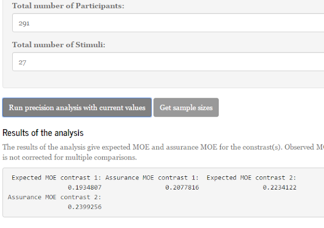
The app promises that using 25 stimuli combined with 290 participants or 25 participants and 290 items will do the trick (the symmetry of these results are due to the fact that the interaction components are equal; both the treatment by participant and the treatment by stimulus interaction component equal .10). Since we have 3 treatment conditions using 290 participants or stimuli is a little awkward, so I suggest to use 291 (equals 97 participants per group or 97 items per list). (300 is a much nicer figure of course). Likewise, as it is hard to equally divide 25 stimuli or participants over three lists or groups, use a multiple of three (say: 27).

If we input the suggest sample sizes in the app, we see the following results if we choose the run precision analysis with current values.

As you can see: Assurance MOE is close to 0.25 (.24) for the second contrast (the least precise one), so 80% of replication experiments will get estimated MOE of 0.25 (.24) or smaller. The expected precision is 0.22. The first contrast (which can be estimated with more precision) has assurance MOE of 0.21 and expected MOE of approximately 0.19. Thus, the sample sizes lead to the results we want.

References

Cumming, G. (2012). Understanding the New Statistics. New York/London: Routledge.

Sahai, H., & Ageel, M. I. (2000). The analysis of variance. Fixed, Random, and Mixed Models. Boston/Basel/Berlin: Birkhäuser.

Westfall, J., Kenny, D. A., & Judd, C. M. (2014). Statistical power and optimal design in experiments in which samples of participants respond to samples of stimuli. Journal of Experimental Psychology: General, 143(5), 2020-2045.