In a previous post, which can be found here, I described how the relative error variance of a treatment mean can be obtained by combining variance components. I concluded that post by mentioning how this relative error variance for the treatment mean can be used to obtain the variance of a contrast estimate. In this post, I will discuss a little more how this latter variance can be used to obtain a confidence interval for the contrast estimate, but we take a few steps back and consider a relatively simple study.
The plan of this post is as follows. We will have a look at the analysis of a factorial design and focus on estimating an interaction effect. We will consider both the NHST approach and an estimation approach. We will use both ‘hand calculations’ and SPSS.
An important didactic aspect of this post is to show the connection between the ANOVA source table and estimates of the standard error of a contrast estimate. Understanding that connections helps in understanding one of my planned posts on how obtaining these estimates work in the case of mixed model ANOVA. See the final section of this post.
The data we will be analyzing are made up. They were specifically designed for an exam in one of the undergraduate courses I teach. The story behind the data is as follows.
Description of the study
A researcher investigates the extent to which the presence of seductive details in a text influences text comprehension and motivation to read the text. Seductive details are pieces of information in a text that are included to make the text more interesting (for instance by supplying fun-facts about the topic of the text) in order to increase the motivation of the reader to read on in the text. These details are not part of the main points in the text. The motivation to read on may lead to increased understanding of the main points in the text. However, readers with much prior knowledge about the text topic may not profit as much as readers with little prior knowledge with respect to their understanding of the text, simply because their prior knowledge enables them to comprehend the text to an acceptable degree even without the presence of seductive details.
The experiment has two independent factors, the readers’ prior knowledge (1 = Little, 2 = Much) and the presence of seductive details (1 = Absent, 2 = Present) and two dependent variables, Text comprehension and Motivation. The experiment has a between participants design (i.e. participant nested within condition).
The research question is how much the effect of seductive details differs between readers with much and readers with little prior knowledge. This means that we are interested in estimating the interaction effect of presence of seductive details and prior knowledge on text comprehension.
The NHST approach
In order to appreciate the different analytical focus between traditional NHST (as practiced) and an estimation approach, we will first take a look at the NHST approach to the analysis. It may be expected that researchers using that approach perform an ANOVA ritual as a means of answering the research question. Their focus will be on the statistical significance of the interaction effect, and if that interaction is significant the effect of seductive details will be investigated separately for participants with little and participants with much prior knowledge. The latter analysis focuses on whether these simple effects are significant or not. If the interaction effect is not significant, it will be concluded that there is no interaction effect. Of course, besides the interaction effect, the researcher performing the ANOVA ritual will also report the significance of the main effects and will conclude that main effects exist or not exist depending on whether they are significant or not. The more sophisticated version of NHST will also include an effect size estimate (if the corresponding significance test is significant) that is interpreted using rules of thumb.
The two way ANOVA output (including partial eta squared) is as follows.
 |
| Table 1. Output of traditional two-way ANOVA |
The results of the analysis will probably be reported as follows.
There was a significant main effect of prior knowledge (F(1, 393) = 39.26, p < .001, partial η2 = .09). Participants with much prior knowledge had a higher mean text comprehension score than the participants with little prior knowledge. There was no effect of the presence of seductive details (F < 1). The interaction effect was significant (F(1, 393) = 4.33, p < .05, partial η2 = .01).
Because of the significant interaction effect, simple effects analyses were performed to further investigate the interaction. These results show a significant effect of the presence of seductive details for the participants with little knowledge (p < .05), with a higher mean score in the condition with seductive details, but for the participants with much prior knowledge no effect of seductive details was found (p = .38), which explains the interaction. (Note: with a Bonferroni correction for the two simple effects analyses the p-values are p = .08 and p = .74; this will be interpreted as that neither readers with little knowledge nor with much knowledge benefit from the presence of seductive details).
The conclusion from the traditional analysis is that the effect of seductive details differs between readers with little and readers with much prior knowledge. The presence of seductive details only has an effect on the comprehension scores of readers with little prior knowledge of the text topic, in the presence of seductive details text comprehension is higher than in the absence of seductive details. Readers with much prior knowledge do not benefit from the presence of seductive details in a text.
Comment on the NHST analysis
The first thing to note is that the NHST conclusion does not really answer the research question. Whereas the research question ask how much the effects differ, the answer to the research question is that a difference exists. This answer is further specified as that there exists an effect in the little knowledge group, but that there is no effect in the much knowledge group.
The second thing to note is that although there is a simple research questions, the report of the results includes five significance tests, while none of them actually address the research question. (Remember it is an how-much question and not a whether-question, the significance tests do not give useful information about the how-much question).
The third thing to notice is that although effect sizes estimates are included (for the significant effects only) they are not interpreted while drawing conclusions. Sometimes you will encounter such interpretations, but usually they have no impact on the answer to the research question. That is, the researcher may include in the report that there is a small interaction effect (using rules-of-thumb for the interpretation of partial eta-squared; .01 = small; .06 = medium, .14 = large), but the smallness of the interaction effect does not play a role in the conclusion (which simply reformulates the (non)significance of the results without mentioning numbers; i.e. that the effect exists (or was found) in one group but not in the other).
As an aside, the null-hypothesis test for the effect of prior knowledge i.e. that the mean comprehension score of readers with little knowledge are equal to the mean comprehension score of readers with much prior knowledge about the text topic seems to me an excellent example of a null-hypothesis that is so implausible that rejecting it is not really informative. Even if used as some sort of manipulation check the real question is the extent to which the groups differ and not whether the difference is exactly zero. That is to say, not every non-zero difference is as reassuring as every other non-zero difference: there should be an amount of difference between the groups below which the group performances can be considered to be practically the same. If a significance tests is used at all, the null-hypothesis should specify that minimum amount of difference.
Estimating the interaction effect
We will now work towards estimating the interaction effect. We will do that in a number of steps. First, we will estimate the value of the contrasts on the basis of the estimated marginal means provided by the two-way ANOVA and show how the confidence interval of that estimate can be obtained. Second, we will use SPSS to obtain the contrast estimate.
Table 2 contains the descriptives and samples sizes for the groups and the estimated marginal means are presented in Table 3.
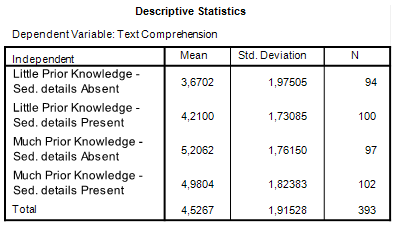 |
| Table 2. Descriptive Statistics |
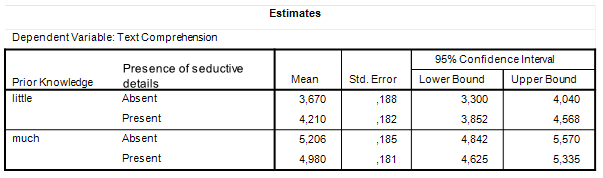 |
| Table 3. Estimated Marginal Means |
Let’s spend a little time exploring the contents of Table 3. The estimated means speak for themselves, hopefully. These are simply estimates of the population means.
The standard errors following the means are used to calculate confidence intervals for the population means. The standard error is based on an estimate of the common population variance (the ANOVA model assumes homogeneity of variance and normally distributed residuals). That estimate of the common variance can be found in Table 1: it is the Mean Square Error. Its estimated value is 3.32, based on 389 degrees of freedom.
The standard errors of the means in Table 3 are simply the square root of the Mean Square Error dvided by the sample size. E.g. the standard error of the mean text comprehension in the group with little knowledge and seductive details absent equals √(3.32/94) = .1879.
The Margin of Error needed to obtain the confidence interval is the critical t-value with 389 degrees of freedom (the df of the estimate of Mean Square Error) multiplied by the standard error of the mean. E.g. the MOE of the first mean is t.975(389)*.1879 = 1.966*.1879 = 0.3694.
The 95%-confidence interval for the first mean is therefore 3.67 +/- 0.3694 = [3.30, 4.04].
Contrast estimate
We want to know the extent to which the effect of seductive details differs between readers with little and much prior knowledge. This means that we want to know the difference between the differences. Thus, the difference between the means of the Present (P) and Absent (A) of readers with Much (M) knowledge is subtracted from the difference between the means of the readers with Little (L) knowledge: (ML+P – ML+A) – (MM+P – MM+A) = ML+P – ML+A – MM+P + MM+A = 4.210 – 3.670 – 4.980 + 5.206 = 0.766.
Our point estimate of the difference between the effect of seductive details for little knowledge readers and for much knowledge is that the effect is 0.77 points larger in the group with little knowledge.
For the interval estimate we need the estimated standard error of the contrast estimate and a critical value for the central t-statistic. To begin with the latter: the degrees of freedom are the degrees of freedom used to estimate Mean Square Error (df = 389; see Table 1).
The standard error of the contrasts estimate can be obtained by using the variance sum law. That is, the variance of the sum of two variables is the sum of their variances plus twice the covariance. And the variance of the difference between two variables is the sum of the variances minus twice the covariance. In the independent design, all the covariances between the means are zero, so the variance of the interaction contrast is simply the sum of the variances over the means. The standard error is the square root of this figure. Thus, var(interaction contrast) = 0.1882 + 0.1822 + 0.1852 + 0.1812 = 0.1354, and the standard error of the contrast is the square root of 0.1354 = .3680.
Note that the we have squared the standard errors of the mean. These squared standard error are the same as the relative error variances of the means. (Actually, in a participant nested under treatment condition (a between-subject design) the relative error variance of the mean equals the absolute error variance). More information about the error variance of the mean can be found here: https://the-small-s-scientist.blogspot.nl/2017/05/PFP-variance-components.html.
The Margin of Error of the contrast estimate is therefore t.975(389)*.3680 = 1.966*.3680 = 0.7235. The 95% confidence interval for the contrast estimate is [0.04, 1.49].
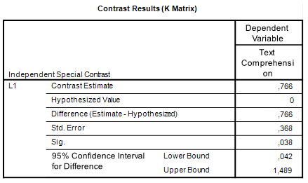
Thus, the answer to the research question is that the estimated difference in effect of seductive details between readers with little prior knowledge and readers with much prior knowledge about the text topic equals .77, 95% CI [.04, 1.49]. The 95% confidence interval shows that the estimate is very imprecise, since the limits of the interval are .04, which suggests that the effect of seductive details is essentially similar for the different groups of readers, and 1.49, which shows that the effect of seductive details may be much larger for little knowledge readers than for much knowledge readers.
Analysis with SPSS
I think it is easiest to obtain the contrast estimate by modeling the data with one-way ANOVA by including a factor I’ve called ‘independent’. (Note: In this simple case, the parameter estimates output of the independent factorial ANOVA also gives the interaction contrast (including the 95% confidence interval), so there is no actual need to specify contrasts, but I like to have the flexibility of being able to get an estimate that directly expresses what I want to know). This factor has 4 levels: one for each of the combinations of the factors prior knowledge and presence of seductive details: Little-Absent (LA), Little-Present (LP), Much-Absent (MA), and Much-Present (MP).
The interaction we’re after is the difference between the mean difference between Present and Absent for participants with little knowledge (MLP – MLA) and the mean difference between Present and Absent in the much knowledge group (MMP – MMA). Thus, the estimate of the interaction (difference between differences) is (MLP – MLA) – (MMP – MMA) = MLP – MLA – MMP + MMA. This can be rewritten as 1*MLP + -1*MLA + -1*MMP + 1*MMA).
The 1’s and -1’s are of course the contrast weights we have to specify in SPSS in order to get the estimate we want. We will have to make sure that the weights correspond to the way in which the order of the means is represented internally in SPSS. That order is LA, LP, MA, MP. Thus, the contrast weights need to be specified in that order to get the estimate to express what we want in terms of the difference between differences. See the second line in the following SPSS-syntax.
UNIANOVA comprehension BY independent
/CONTRAST(independent)=SPECIAL ( -1 1 1 -1)
/METHOD=SSTYPE(3)
/INTERCEPT=INCLUDE
/EMMEANS=TABLES(independent)
/PRINT=DESCRIPTIVE
/CRITERIA=ALPHA(.05)
/DESIGN=independent.
The relevant output is presented in Table 4. Note that the results are the same as the ‘hand calculations’ described above (I find this very satisfying).
 |
| Table 4. Interaction contrast estimate |
Comment on the analysis
First note that the answer to the research question has been obtained with a single analysis. The analysis gives us a point estimate of the difference between the differences and a 95% confidence interval. The analysis is to the point to the extent that it gives the quantitative information we seek.
However, although the estimate of the difference between the differences is all the quantitative information we need to answer the how-much-research question, the estimate itself obscures the pattern in the results, in the sense that the estimate itself does not tell us what may be important for theoretical or practical reasons, namely the direction of the effect. That is, a positive interaction contrast may indicate the difference between an estimated positive effect for one group and an estimated negative effect in the other group (which is actually the situation in the present example: 0.54 – (-0.23) = 0.77) in the other group).
Of course, we could argue that if you want to know the extent to which the size and direction differ between the groups, then that should be reflected in your research question, for instance, by asking about and estimating the simple effects themselves in stead of focusing on the size of the difference alone, as we have done here.
On the other hand, we could argue that no result of a statistical analysis should be interpreted in isolation. Thus, there is no problem with interpreting the estimate of 0.77 while referring to the simple effects: the estimated difference between the effects is .77, 95% CI [.04, 1.49], reflecting the difference between an estimated effect of 0.54 in the little knowledge group and an estimated negative effect of -0.23 for much knowledge readers.
But, if the research question is how large is the effect of seductive details for little knowledge readers and high knowledge readers and how much do the effect differ, than that would call for three point estimates and interval estimates. Like: the estimated effect for the little knowledge group equals 0.54. 95% CI [0.03, 1.06], whereas the estimated effect for the much knowledge groups is negative -0.23, 95% CI [-0.73, 0.28]. The difference in effect is therefore 0.77, 95% CI [.04, 1.49].
In all cases, of course, the intervals are so wide that no firm conclusions can be drawn. Consistent with the point estimates are negligibly small positive effects to large positive effects of seductive details for the little knowledge group, small positive effects to negative effects of seductive details for the much knowledge group and an interaction effect that ranges from negligibly small to very large. In other words, the picture is not at all clear. (Interpretations of the effect sizes are based on rules of thumb for Cohen’s d. A (biased) estimate of Cohen’s d can be obtained by dividing the point estimate by the square root of Mean Square Error. An approximate confidence interval can be obtained by dividing the end-points of the non-standardized confidence intervals by the square root of Mean Square Error). Of course, we have to keep in mind that 5% of the 95% confidence intervals do not contain the true value of the parameter or contrast we are estimating.
Compare this to the firm (but unwarranted) NHST conclusion that there is a positive effect of seductive details for little knowledge readers (we don’t know whether there is a positive effect, because we can make a type I error if we reject the null) and no effect for much knowledge readers. (Yes, I know that the NHST thought-police forbids interpreting non-significant results as “no effect”, but we are talking about NHST as practiced and empirical research shows that researchers interpret non-significance as no effect).
In any case, the wide confidence intervals show that we could do some work for a replication study in terms of optimizing the precision of our estimates. In a next post, I will show you how we can use our estimate of precision for planning that replication study.
Summary of the procedure
In (one of the next) posts, I will show that in the case of mixed models ANOVA’s we frequently need to estimate the degrees of freedom in order to be able to obtain MOE for a contrast. But the basic logic remains the same as what we have done in estimating the confidence interval for the interaction contrast. Please keep in mind the following.
Looking at the ANOVA source table and the traditional ANOVA approach we notice that the interaction effect is tested against Mean Square Error: the F-ratio we use to test the null-hypothesis that both Mean Squares (the interaction MS an Mean Square Error) estimate the common error variance. The F-ratio is formed by dividing the Mean Square associated with the interaction by Mean Square Error. The probability distribution of that ratio is an F-distribution with 1 (numerator) and 389 (denominator) degrees of freedom.
Mean Square Error is also used to obtain the estimated standard error for the interaction contrast estimate. In the calculation of MOE, the critical value of t was determined on the basis of the degrees of freedom of Mean Square Error.
This is the case in general: the standard error of a contrast is based on the Mean Square Error that is also used to test the corresponding Effect (main or interaction) in an F-test. In a simple two-way ANOVA the same Mean Square Error is used to test all the effects (main an interaction), but that is not generally the case for more complex designs. Also, the degrees of freedom used to obtain a critical t-value for the calculation of MOE are the degrees of freedom of the Mean Square Error used to test an effect.
In the case of a mixed model ANOVA, it is often the case that there is no Mean Square Error available to directly test an effect. The consequence of this is that we work with linear combinations of Mean Squares to obtain a suitable Mean Square Error for an effect and that we need to estimate the degrees of freedom. But the general logic is the same: the Mean Square Error that is obtained by a linear combination of Mean Squares is also used to obtain the standard error for the contrast estimate and the estimated degrees of freedom are the degrees of freedom used to obtain a critical value for t in the calculation of the Margin of Error.
I will try to write about all of that soon.


 . Now, suppose that due to some freak accident of nature there are no differences in the mean scores (averaged of stimuli) of each participant. In that case,
  . This means that under these circumstances the expected mean square associated with participants is simply an estimate of the error variance with
  degrees of freedom, because
  , if
, if  degrees of freedom. The logic of the F-test is that under the null-hypothesis, in our case that
  . If we now suppose that there is no difference between the treatment means, that is
  , MSTreatment does not estimate
  , but
, but  . Note that no other source of variance has an expected mean square that is equal to the latter figure. That is, in contrast to our test of the Participant factor, where under the null-hypotheses two Mean Squares estimate the error variance, i.e. MSParticipant and MSError, no mean square is available to form an F-ratio to test the Treatment effect.
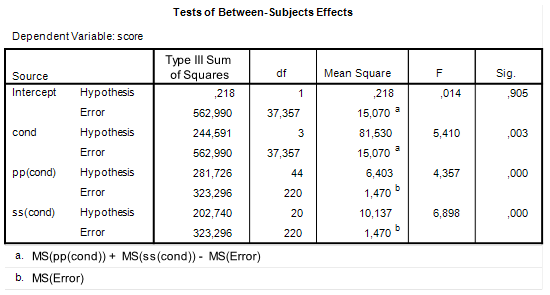
![[m\sigma^2_p + \sigma^2_e] + [m\sigma^2_s + \sigma^2_e] - [\sigma^2_e] = m\sigma^2_p + n\sigma^2_s + \sigma^2_e](https://small-s.science/wp-content/ql-cache/quicklatex.com-9cd6bb15506816413e74641fee23cf13_l3.png "Rendered by QuickLaTeX.com") . It is exactly this linear combination of mean squares that is used in the F-ratio to obtain an error term against which to test the Treatment effect in Figure 1:
. It is exactly this linear combination of mean squares that is used in the F-ratio to obtain an error term against which to test the Treatment effect in Figure 1:  . We will also use this figure to obtain the variance (and standard error) of our contrast estimate.
![\[df=\frac{(MSp+MSs-MSe)^{2}}{\frac{MSp^{2}}{df_{p}}+\frac{MSs^{2}}{df_{s}}+\frac{MSe^{2}}{df_{e}}}.\]](https://small-s.science/wp-content/ql-cache/quicklatex.com-13f753be88a6e13890953c2465e22a05_l3.png "Rendered by QuickLaTeX.com")
 can be obtained as follows.
![\[\hat{\sigma}_{\hat{\psi}}=\sqrt{\sum c_{i}^{2}\hat{\sigma}_{\bar{X},Rel}^{2}},\]](https://small-s.science/wp-content/ql-cache/quicklatex.com-489e315828278a9811848f3ce71bf10f_l3.png "Rendered by QuickLaTeX.com")
 to refer to the relative error variance of the treatment mean (which in this design is equal to the absolute error variance, but that’s another story), and
  refers to the contrast weight of treatment mean i. The relative error variance of the treatment mean is obtained by dividing the error variance that is used to test the treatment effect by the total number of observations in each treament,
  . Thus, using the results in Figure 1.
![\[\hat{\sigma}_{\bar{X},Rel}^{2}=\frac{MS_{p}+MS_{s}-MS_{e}}{nm}=\frac{15.07}{72}=0.2093.\]](https://small-s.science/wp-content/ql-cache/quicklatex.com-0d81fe2ec65ea2c26c84682713e499bf_l3.png "Rendered by QuickLaTeX.com")
 . Let’s use the results in Figure 1 to calculate what MOE is for this particular contrast.
 , with 220 degrees of freedom and not
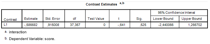
  , with 37.357 (see Figure 1). The consequence of this is, of course, that the 95% CI is much narrower than it should be.
 , the critical value of t is the .975 quantile of the central t distribution with
  , which equals
  . The value of MOE is therefore
  . With a contrast estimate of
  , the 95% CI equals
 ![-0.587 \pm 0.5633 = [-1.1503, -0.0237]](https://small-s.science/wp-content/ql-cache/quicklatex.com-ea5612615f1baf096374644a223d775f_l3.png "Rendered by QuickLaTeX.com") . In comparison, using the correct value of MOE gives us
. In comparison, using the correct value of MOE gives us ![[−2.4404, 1.2664]](https://small-s.science/wp-content/ql-cache/quicklatex.com-ef97651e8790dc304790e8a8724ebed7_l3.png "Rendered by QuickLaTeX.com") .
.
 , approximate 95% CI
 ![[-1.40, 0.73]](https://small-s.science/wp-content/ql-cache/quicklatex.com-867264624a612f401b2c1cea536372a9_l3.png "Rendered by QuickLaTeX.com") , which according to the rules of thumb is a medium negative effect, but consistent with anytihing from a huge negative effect to a large positive effect in the population, as the approximate CI shows. (I have divided the point estimate and the confidence interval in Figure 2 by 1.74, to obtain Cohen’s d and an approximate confidence interval). Clearly, then, our precision can be optimized.
, which according to the rules of thumb is a medium negative effect, but consistent with anytihing from a huge negative effect to a large positive effect in the population, as the approximate CI shows. (I have divided the point estimate and the confidence interval in Figure 2 by 1.74, to obtain Cohen’s d and an approximate confidence interval). Clearly, then, our precision can be optimized. , the stimulus variance
  , and the error variance
  . Rearranging and using 1.47 as an estimate for
  . Likewise, the estimate for
  . Thus, our estimates are
  ,
,  , and
, and  .
.
 , for assurance the value .80 and the values
  , and
, and  for, respectively, Residual variance, Participant intercept variance and Stimulus intercept variance. Fill in the value 0 for all the other variances. See Figure 5.

 , to refer to the residual variance in the BwC-design, we can say
  . Normally, the precision app sums these two components to get a value for the residual variance in the BwC-design, and you will obviously get the same result if you specify the residual variance as the sum and the participant-by-stimulus variance as 0. Likewise,
  , and
, and  , where
  and
and  are the variances associated with the interaction of treatment and participant and treatment and stimulus, respectively.
 , and there is 80% assurance that MOE will not exceed
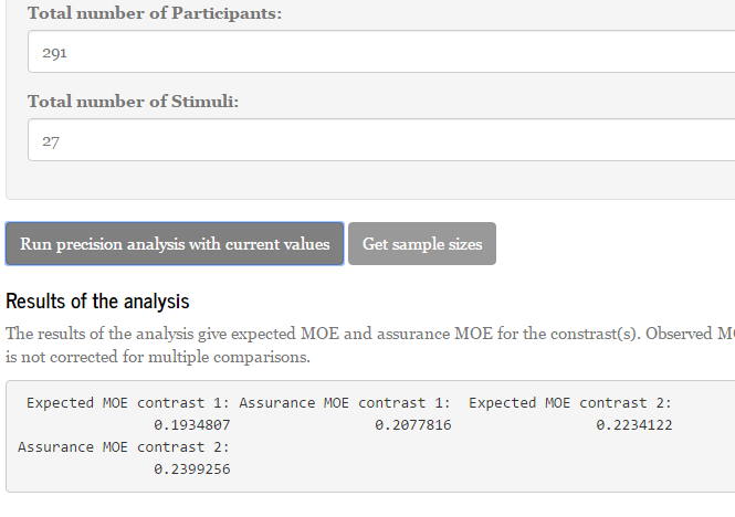
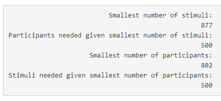
  . Note, again, that the assurance MOE is somewhat larger than target MOE, because a sample of 804 participants requires a sample of more than 500 stimuli to get the target MOE with 80% assurance and 500 stimuli is the maximum number of stimuli the app considers when minimizing the number of participants.

 ,
,  ,
,  ,
,  ,
,  , and
, and  . The Satterthwaite degrees of freedom are
  . The standard error of the contrast equals
  . The critical value for t equals
  . Expected MOE is, therefore,
  (the tiny difference with the results from the app is due to rounding errors).
 -distribution. That is, we assume with assurance
  , that the
  . Now, the degrees of freedom are
  , the assurance
  , and the .80 quantile of
  . Since the relative error variance equals
  , the .80 quantile of the error variance equals
  . And this means that assurance MOE equals
  . Again, the difference with the results from the Precision App are due to rounding error.
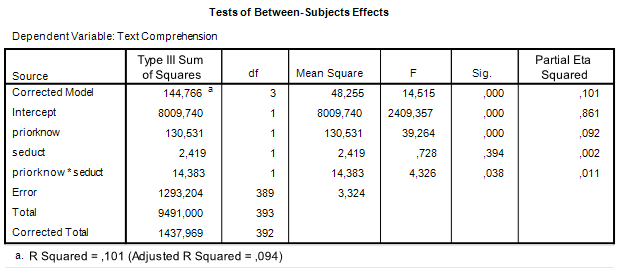
![\[\hat{\sigma_\psi}= \sqrt{\sum{c_i^2MS_e/n_i}},\]](https://small-s.science/wp-content/ql-cache/quicklatex.com-e711016f1b800409ee4d1632159091d7_l3.png "Rendered by QuickLaTeX.com")
 the number of observations (in our example participants) in treatment condition i. Note that
  is the variance of treatment mean i, the square root of which gives the familiar standard error of the mean.
![\[MOE = t_{.975}(df_e)\sqrt{\sum{c_i^2MS_e/n_i}}=t_{.975}(df_e)\sqrt{4MS_e/n_i} = 2t_{.975}(df_e)\sqrt{MS_e/n_i}.\]](https://small-s.science/wp-content/ql-cache/quicklatex.com-c566353662177824c69974b4d59785d4_l3.png "Rendered by QuickLaTeX.com")
 , and the true value of Mean Square Error is 3.324, then MOE for the contrast estimate equals
![\[MOE = 2*t_{.975}(396)*\sqrt{3.324/100} = 0.7071\]](https://small-s.science/wp-content/ql-cache/quicklatex.com-98e408fbb1899034420a41dc86f58115_l3.png "Rendered by QuickLaTeX.com")
![\[MOE = 2*t_{.975}(df_e)\sqrt{(MS_w / n_i)},\]](https://small-s.science/wp-content/ql-cache/quicklatex.com-1984a751953fc6b0698d72e7bf2c550b_l3.png "Rendered by QuickLaTeX.com")
 , since we are considering the 2×2 design.
![\[0.4558 = 2*t_{.975}(4(n_i - 1)\sqrt{(MS_w / n_i)},\]](https://small-s.science/wp-content/ql-cache/quicklatex.com-9a775e47b691309421ea2f9d94c016c2_l3.png "Rendered by QuickLaTeX.com")
![\[MOE_{\gamma} = 2*t_{.975}(df)*\sqrt{MS_w/n_i*\chi^2_{\gamma}(df)/df},\]](https://small-s.science/wp-content/ql-cache/quicklatex.com-f5945fe8ef0dad8f2bf28d70a7553fae_l3.png "Rendered by QuickLaTeX.com")
 is the assurance expressed in a probability between 0 and 1.


![\[E(MOE) = t_{.975}(df)*\sigma_{\hat{\psi}},\]](https://small-s.science/wp-content/ql-cache/quicklatex.com-3c365ea8bf332e7cfe0131922eaadfca_l3.png "Rendered by QuickLaTeX.com")
 is the standard error of the contrast estimate. Of course, both the standard error and the df are functions of the sample sizes.
 , where a is the number of treatment conditions, we use the following general expression.
![\[\sigma_{\hat{\psi}} = \sqrt{\sum c^2_i \frac{\sigma^2_w}{n}},\]](https://small-s.science/wp-content/ql-cache/quicklatex.com-2047baef6bfe75fa33fdb76808ad99fe_l3.png "Rendered by QuickLaTeX.com")
 the within treatment variance (we assume homogeneity of variance).
 and
and  , and
, and  , the standard error for this contrast equals
  . (Note that this is simply the standard error of the difference between two means as used in the independent samples t-test).
 . The expected MOE for this design is therefore,
  . Note that using these figures entails that 95% of the contrast estimates will take values between the true contrast value plus and minus the expected MOE:
  .
. }, the same sample sizes and within treatment variance gives
  .
.![\[MS_w \sim \sigma^2_w*\chi^2(df)/df,\]](https://small-s.science/wp-content/ql-cache/quicklatex.com-33d9394fa378a467d81b18b1eebf8d8d_l3.png "Rendered by QuickLaTeX.com")
![\[\hat{MOE} \sim t_{.975}(df)\sqrt{\frac{1}{n}\sum{c_i^2}\sigma^2_w*\chi^2(df)/df}.\]](https://small-s.science/wp-content/ql-cache/quicklatex.com-55d2923233b4c1800935a900bed6c86c_l3.png "Rendered by QuickLaTeX.com")
![\[\hat{MOE}_{.80} = 2.0244 * \sqrt{1/20*2*20*45.07628/38} = 3.1181.\]](https://small-s.science/wp-content/ql-cache/quicklatex.com-7389e9cdfe17c1809754f3a5cdf0962f_l3.png "Rendered by QuickLaTeX.com")
 in the chi-squared (df = 38) distribution. That is
  .
. , and the number of observations in each group by list combination equals
  . The condition means are estimated by combining a group by list combinations each of which composed of different participants and stimuli. The total number of observations per condition is therefore,
  .
.![\[Y_{ijk} = \mu + \alpha_i + \beta_j + \gamma_k + (\alpha\beta)_{ij} + (\alpha\gamma)_{ik} + e_{ijk},\]](https://small-s.science/wp-content/ql-cache/quicklatex.com-0fe0fded4cedc1ede78c9f5dcd9c1c61_l3.png "Rendered by QuickLaTeX.com")
 is a constant treatment effect (it’s a fixed effect), and the other effect are random effects with zero mean and variances
  (participants),
  (items),
  (person by treatment interaction),
  (item by treatment interaction) and
 ![[\sigma^2_{\beta\gamma} + \sigma^2_e]](https://small-s.science/wp-content/ql-cache/quicklatex.com-04ba4ecdae4334a2a41e0f4ab3c241f2_l3.png "Rendered by QuickLaTeX.com") .
. , and
, and  . The latter two restrictions make the interaction-effects correlated across conditions (i,e. the effects of person and treatment are correlated across condition for the same person, likewise the interaction effects of item and treatment are correlated across conditons for the same item. Interaction effects of different participants and items are uncorrelated). The covariances between the random effects
  are assumed to be zero.
 , and
, and  . Furthermore, the covariance of the interactions between treatment and participant or between treatment and item for the same participant or item are
  for participants and
  for items.
 ). Thus,
 ![\sigma^2_w = \frac{q}{a}\sigma^2_{\alpha\beta} + \frac{p}{a}\sigma^2_{\alpha\gamma}+[\sigma^2_{\beta\gamma} + \sigma^2_e]](https://small-s.science/wp-content/ql-cache/quicklatex.com-6a8143341552d56735cb6827e1d9d309_l3.png "Rendered by QuickLaTeX.com") . Note that the latter equals the sum of the expected mean squares of the Treatment by Participant (
. Note that the latter equals the sum of the expected mean squares of the Treatment by Participant ( ) and the Treatment by Item (
 ) interactions, minus the expected mean square associated with Error (
 ).
).![\[df =\frac{(E(MS_{tp}) + E(MS_{ti}) - E(MS_e))^2}{\frac{E(MS_{tp})^2}{(a - 1)(p-a)}+\frac{E(MS_{ti})^2}{(a - 1)(q-a)}+\frac{E(MS_e)^2}{(p-a)(q-a)}}\]](https://small-s.science/wp-content/ql-cache/quicklatex.com-9d20ad417c928f844eff686d67e11de2_l3.png "Rendered by QuickLaTeX.com")
![\[E(MOE) = t(df)*\sqrt{(\sum_{i=1}^a c^2_i)(\frac{1}{a}pq)^{-1}\sigma^2_w}\]](https://small-s.science/wp-content/ql-cache/quicklatex.com-c0d601b03e80c69eaa13d78d5fa26d94_l3.png "Rendered by QuickLaTeX.com")
![\[= t(df)*\sqrt{(\sum_{i=1}^a c^2_i)(\frac{1}{a}pq)^{-1}(\frac{q}{a}\sigma^2_{\alpha\beta} + \frac{p}{a}\sigma^2_{\alpha\gamma}+[\sigma^2_{\beta\gamma} + \sigma^2_e])}\]](https://small-s.science/wp-content/ql-cache/quicklatex.com-9d1fd09440d619a3e308d67a14f6d5af_l3.png "Rendered by QuickLaTeX.com")
![\[=t(df)*\sqrt{(\sum_{i=1}^a c^2_i)(pq)^{-1}(q\sigma^2_{\alpha\beta} + p\sigma^2_{\alpha\gamma}+a[\sigma^2_{\beta\gamma} + \sigma^2_e])}\]](https://small-s.science/wp-content/ql-cache/quicklatex.com-1fdcd788de0cbf5b0b33af1de00e8594_l3.png "Rendered by QuickLaTeX.com")
![\[=t(df)*\sqrt{(\sum_{i=1}^a c^2_i)(\sigma^2_{\alpha\beta}/p + \sigma^2_{\alpha\gamma}/q +a[\sigma^2_{\beta\gamma} + \sigma^2_e]/pq)}\]](https://small-s.science/wp-content/ql-cache/quicklatex.com-a6d07edd78ffac88f7f956fe4b50dcdd_l3.png "Rendered by QuickLaTeX.com")
 . Suppose furthermore, that 10% of the variance can be attributed to treatment by participant interaction, 10% of the variance to the treatment by item interaction and 40% of the variance to the error confounded with the participant by item interaction. (which leaves 40% of the total variance attributable to participant and item variance.
 ,
,  , and
, and  . Our target MOE is .25, and we plan to use the counterbalanced design with p = 30 participants, and q = 15 items (stimuli).
 ,
,  , and
, and  , and the approximate df equal
  .
. .
.