Many experiments involve the (quasi-)random selection of both participants and items. Westfall et al. (2014) provide a Shiny-app for power-calculations for five different experimental designs with selections of participants and items. Here I want to present my own Shiny-app for planning for precision of contrast estimates (for the comparison of up to four groups) in these experimental designs. The app can be found here: https://gmulder.shinyapps.io/precision/
(Note: I have taken the code of Westfall’s app and added code or modified existing code to get precision estimates in stead of power; so, without Westfall’s app, my own modified version would never have existed).
The plan for this post is as follows. I will present the general theoretical background (mixed model ANOVA combined with ideas from Generalizability Theory) by considering comparing three groups in a counter balanced design.
Note 1: This post uses mathjax, so it’s probably unreadable on mobile devices. Note: a (tidied up) version (pdf) of this post can be downloaded here: download the pdf
Note 2: For simulation studies testing the procedure go here: https://the-small-s-scientist.blogspot.nl/2017/05/planning-for-precision-simulation.html
Note 3: I use the terms stimulus and item interchangeably; have to correct this to make things more readable and comparable to Westfall et al. (2014).
Note 4: If you do not like the technical details you can skip to an illustration of the app at the end of the post.
The general idea
The focus of planning for precision is to try to minimize the half-width of a 95%-confidence interval for a comparison of means (in our case). Following Cumming’s (2012) terminology I will call this half-width the Margin of Error (MOE). The actual purpose of the app is to find required sample sizes for participants and items that have a high probability (‘assurance’) of obtaining a MOE of some pre-specified value.
Expected MOE for a contrast
For a contrast estimate  we have the following expression for the expected MOE.
![\[E(MOE) = t_{.975}(df)*\sigma_{\hat{\psi}},\]](https://small-s.science/wp-content/ql-cache/quicklatex.com-3c365ea8bf332e7cfe0131922eaadfca_l3.png "Rendered by QuickLaTeX.com")
where  is the standard error of the contrast estimate. Of course, both the standard error and the df are functions of the sample sizes.
For the standard error of a contrast with contrast weights  through
  , where a is the number of treatment conditions, we use the following general expression.
![\[\sigma_{\hat{\psi}} = \sqrt{\sum c^2_i \frac{\sigma^2_w}{n}},\]](https://small-s.science/wp-content/ql-cache/quicklatex.com-2047baef6bfe75fa33fdb76808ad99fe_l3.png "Rendered by QuickLaTeX.com")
where n is the per treatment sample size (i.e. the number of participants per treatment condition times the number of items per treatment condition) and  the within treatment variance (we assume homogeneity of variance).
For a simple example take an independent samples design with n = 20 participants responding to 1 item in one of two possible treatment conditions (this is basically the set up for the independent t-test). Suppose we have contrast weights  and
and  , and
, and  , the standard error for this contrast equals
  . (Note that this is simply the standard error of the difference between two means as used in the independent samples t-test).
In this simple example, df is the total sample size (N = n*a) minus the number of treatment conditions (a), thus  . The expected MOE for this design is therefore,
  . Note that using these figures entails that 95% of the contrast estimates will take values between the true contrast value plus and minus the expected MOE:
  .
.
For the three groups case, and contrast weights { }, the same sample sizes and within treatment variance gives
  .
.
(If you like, I’ve written a little document with derivation of the variance of selected contrast estimates in the fully crossed design for the comparison of two and three group means. That document can be found here: https://drive.google.com/open?id=0B4k88F8PMfAhaEw2blBveE96VlU)
The focus of planning for precision is to try to find sample sizes that minimize expected MOE to a certain target MOE. The app uses an optimization function that minimizes the squared difference between expected MOE and target MOE to find the optimal (minimal) sample sizes required.
Planning with assurance
If the expected MOE is equal to target MOE, the sample estimate of MOE will be larger than your target MOE in 50% of replication experiments. This is why we plan with assurance (terminology from Cumming, 2012). For instance, we may want to have a 95% probability (95% assurance) that the estimated MOE will not exceed our target MOE.
In order to plan with assurance, we need (an approximation of) the sampling distribution of MOE. In the ANOVA approach that underlies the app, this boils down to the distribution of estimates of :
![\[MS_w \sim \sigma^2_w*\chi^2(df)/df,\]](https://small-s.science/wp-content/ql-cache/quicklatex.com-33d9394fa378a467d81b18b1eebf8d8d_l3.png "Rendered by QuickLaTeX.com")
thus
![\[\hat{MOE} \sim t_{.975}(df)\sqrt{\frac{1}{n}\sum{c_i^2}\sigma^2_w*\chi^2(df)/df}.\]](https://small-s.science/wp-content/ql-cache/quicklatex.com-55d2923233b4c1800935a900bed6c86c_l3.png "Rendered by QuickLaTeX.com")
In terms of the two-groups independent samples design above: the expected MOE equals 2.8629. But, with df = 38, there is an 80% probability (assurance) that the estimated MOE will be no larger than:
![\[\hat{MOE}_{.80} = 2.0244 * \sqrt{1/20*2*20*45.07628/38} = 3.1181.\]](https://small-s.science/wp-content/ql-cache/quicklatex.com-7389e9cdfe17c1809754f3a5cdf0962f_l3.png "Rendered by QuickLaTeX.com")
Note that the 45.07628 is the quantile  in the chi-squared (df = 38) distribution. That is
  .
.
The app let’s you specify a target MOE and a value for the desired assurance ( ) and will find the combination of number of participants and items that will give an estimated MOE no larger than target MOE in % of the replication experiments.
The mixed model ANOVA approach
Basically, what we need to plan for precision is to able to specify and the degrees of freedom. We will specify as a function of variance components and use the Satterthwaite procedure to approximate the degrees of freedom by means of a linear combination of expected mean squares. I will illustrate the approach with a three-treatment conditions counterbalanced design.
A description of the design
Suppose we are interested in estimating the differences between three group means. We formulate two contrasts: one contrast estimates the mean difference between the first group and the average of the means of the second and third groups. The weights of the contrasts are respectively {1, -1/2, -1/2}, and {0, 1, -1}.
We are planning to use a counterbalanced design with a number of participants equal to p and a sample of items of size q. In the design we randomly assign participants to a groups, where a is the number of conditions, and randomly assign items to a lists (see Westfall et al., 2014 for more details about this design). All the groups are exposed to all lists of stimuli, but the groups are exposed to different lists in each condition. The number of group by list combinations equals  , and the number of observations in each group by list combination equals
  . The condition means are estimated by combining a group by list combinations each of which composed of different participants and stimuli. The total number of observations per condition is therefore,
  .
.
The ANOVA model
The ANOVA model for this design is
![\[Y_{ijk} = \mu + \alpha_i + \beta_j + \gamma_k + (\alpha\beta)_{ij} + (\alpha\gamma)_{ik} + e_{ijk},\]](https://small-s.science/wp-content/ql-cache/quicklatex.com-0fe0fded4cedc1ede78c9f5dcd9c1c61_l3.png "Rendered by QuickLaTeX.com")
where the effect  is a constant treatment effect (it’s a fixed effect), and the other effect are random effects with zero mean and variances
  (participants),
  (items),
  (person by treatment interaction),
  (item by treatment interaction) and
  (error variance confounded with the person by item interaction). Note: in Table 1 below, is (for technical reasons not important for this blogpost) presented as this confounding
 ![[\sigma^2_{\beta\gamma} + \sigma^2_e]](https://small-s.science/wp-content/ql-cache/quicklatex.com-04ba4ecdae4334a2a41e0f4ab3c241f2_l3.png "Rendered by QuickLaTeX.com") .
.
We make use of the following restrictions (Sahai & Ageel, 2000):  , and
, and  . The latter two restrictions make the interaction-effects correlated across conditions (i,e. the effects of person and treatment are correlated across condition for the same person, likewise the interaction effects of item and treatment are correlated across conditons for the same item. Interaction effects of different participants and items are uncorrelated). The covariances between the random effects
  are assumed to be zero.
Under this model (and restrictions)  , and
, and  . Furthermore, the covariance of the interactions between treatment and participant or between treatment and item for the same participant or item are
  for participants and
  for items.
Within treatment variance
In order to obtain an expectation for MOE, we take the expected mean squares to get an expression or the expected within treatment variance . These expected means squares are presented in Table 1.
The expected within treatment variance can be found in the Treatment row in Table 1. It is comprised of all the components to the right of the component associated with the treatment effect ( ). Thus,
 ![\sigma^2_w = \frac{q}{a}\sigma^2_{\alpha\beta} + \frac{p}{a}\sigma^2_{\alpha\gamma}+[\sigma^2_{\beta\gamma} + \sigma^2_e]](https://small-s.science/wp-content/ql-cache/quicklatex.com-6a8143341552d56735cb6827e1d9d309_l3.png "Rendered by QuickLaTeX.com") . Note that the latter equals the sum of the expected mean squares of the Treatment by Participant (
. Note that the latter equals the sum of the expected mean squares of the Treatment by Participant ( ) and the Treatment by Item (
 ) interactions, minus the expected mean square associated with Error (
 ).
).
Degrees of freedom
The second ingredient we need in order to obtain expected MOE are the degrees of freedom that are used to estimate the within treatment variance. In the ANOVA approach the within treatment variance is estimated by a linear combination of mean squares (as described in the last sentence of the previous section. This linear combination is also used to obtain approximate degrees of freedom using the Satterthwaite procedure:
-
![\[df =\frac{(E(MS_{tp}) + E(MS_{ti}) - E(MS_e))^2}{\frac{E(MS_{tp})^2}{(a - 1)(p-a)}+\frac{E(MS_{ti})^2}{(a - 1)(q-a)}+\frac{E(MS_e)^2}{(p-a)(q-a)}}\]](https://small-s.science/wp-content/ql-cache/quicklatex.com-9d20ad417c928f844eff686d67e11de2_l3.png "Rendered by QuickLaTeX.com")
Expected MOE
(Note: I can’t seem to get mathjax to generate align environments or equation arrays, so the following is ugly; Note to self: next time use R-studio or Lyx to generate R-html or an equivalent format).
The expected value of MOE for the contrasts in the counter balanced design is:
![\[E(MOE) = t(df)*\sqrt{(\sum_{i=1}^a c^2_i)(\frac{1}{a}pq)^{-1}\sigma^2_w}\]](https://small-s.science/wp-content/ql-cache/quicklatex.com-c0d601b03e80c69eaa13d78d5fa26d94_l3.png "Rendered by QuickLaTeX.com")
Finally an example
Suppose we the scores in three conditions are normally distributed with (total) variances  . Suppose furthermore, that 10% of the variance can be attributed to treatment by participant interaction, 10% of the variance to the treatment by item interaction and 40% of the variance to the error confounded with the participant by item interaction. (which leaves 40% of the total variance attributable to participant and item variance.
Thus, we have  ,
,  , and
, and  . Our target MOE is .25, and we plan to use the counterbalanced design with p = 30 participants, and q = 15 items (stimuli).
Due to the model restrictions presented above we have  ,
,  , and .
The value of is therefore,  , and the approximate df equal
  .
.
For the first contrast, with weights {1, -1/2. -1/2}, then, the Expected value for the Margin of Error is  .
.
For the second contrast, with weights {0, 1, -1}, the Expected value of the Margin of Error is 
Thus, using p = 30 participants, and q = 15 items (stimuli) will not lead to an expected MOE larger than the target MOE of .25.
We can use the app to find the required number of participants and items for a given target MOE. If the number of groups is larger than two, the app uses the contrast estimate with the largest expected MOE to calculate the sample sizes (in the default setting the one comparing only two group means). The reasoning is that if the least precise estimate (in terms of MOE) meets our target precision, the other ones meet our target precision as well.
Using the app
I’ve included lot’ of comments in the app itself, but please ignore references to a manual (does not exist, yet, except in Dutch) or an article (no idea whether or not I’ll be able to finish the write-up anytime soon). I hope the app is pretty straightforward. Just take a look at https://gmulder.shinyapps.io/precision/, but the basic idea is:
– Choose one of five designs
– Supply the number of treatment conditions
– Specify contrast(weights) (or use the default ones)
– Supply target MOE and assurance
– Supply values of variance components (read (e,g,) Westfall, et al, 2014, for more details).
– Supply a number of participants and items
– Choose run precision analysis with current values or
– Choose get sample sizes. (The app gives two solutions: one minimizes the number of participants and the other minimizes the number of stimuli/items). NOTE: the number of stimuli is always greater than or equal to 10 and the number of participants is always greater than or equal to 20.
An illustration
Take the example above. Out target MOE equals .25, and we want insurance of .80 to get an estimated MOE of no larger than .25. We use a counter-balanced design with three conditions, and want to estimate two contrasts: one comparing the first mean with the average of means two and three, and the other contrast compares the second mean with the third mean. We can use the default contrasts.
For the variance components, we use the default values provided by Westfall et al. (2014) for the variance components. These are also the default values in the app (so we don’t need to change anything now).
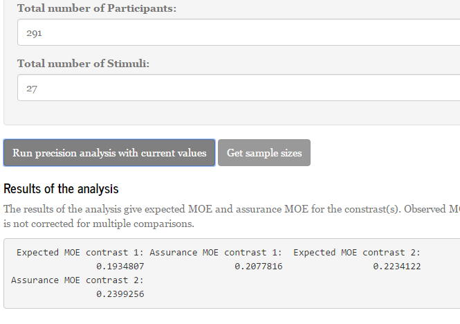
Let’s see what happens when we propose to use p = 30 participants and q = 15 items/stimuli.
Here is part of a screenshot from the app:
These results show that the expected MOE for the first contrast (comparing the first mean with the average of the other means) equals 0.3290, and assurance MOE for the same contrasts equals 0.3576. Remember that we specified the assurance as .80. So, this means that 80% of the replication experiments give estimated MOE as large as or smaller than 0.3576. But we want that to be at most 0.2500. Thus, 30 participants and 15 items do suffice for our purposes.
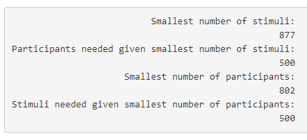
Let’s use to app to get sample sizes. The results are as follows.
The app promises that using 25 stimuli combined with 290 participants or 25 participants and 290 items will do the trick (the symmetry of these results are due to the fact that the interaction components are equal; both the treatment by participant and the treatment by stimulus interaction component equal .10). Since we have 3 treatment conditions using 290 participants or stimuli is a little awkward, so I suggest to use 291 (equals 97 participants per group or 97 items per list). (300 is a much nicer figure of course). Likewise, as it is hard to equally divide 25 stimuli or participants over three lists or groups, use a multiple of three (say: 27).
If we input the suggest sample sizes in the app, we see the following results if we choose the run precision analysis with current values.
As you can see: Assurance MOE is close to 0.25 (.24) for the second contrast (the least precise one), so 80% of replication experiments will get estimated MOE of 0.25 (.24) or smaller. The expected precision is 0.22. The first contrast (which can be estimated with more precision) has assurance MOE of 0.21 and expected MOE of approximately 0.19. Thus, the sample sizes lead to the results we want.
References
Cumming, G. (2012). Understanding the New Statistics. New York/London: Routledge.
Sahai, H., & Ageel, M. I. (2000). The analysis of variance. Fixed, Random, and Mixed Models. Boston/Basel/Berlin: Birkhäuser.
Westfall, J., Kenny, D. A., & Judd, C. M. (2014). Statistical power and optimal design in experiments in which samples of participants respond to samples of stimuli. Journal of Experimental Psychology: General, 143(5), 2020-2045.

![\[\sigma_{\hat{\psi}} = \sqrt{\sum{w_i}\sigma^2_e/n}\]](https://small-s.science/wp-content/ql-cache/quicklatex.com-14bc511e9204319eaaccbcfd696c36c3_l3.png "Rendered by QuickLaTeX.com")
 ) .
) .![\[\sigma^2_e = \sigma^2_{within}(1 - \rho)\]](https://small-s.science/wp-content/ql-cache/quicklatex.com-beec527cea79344408614018693eb04e_l3.png "Rendered by QuickLaTeX.com")

 . Now, suppose that due to some freak accident of nature there are no differences in the mean scores (averaged of stimuli) of each participant. In that case,
  . This means that under these circumstances the expected mean square associated with participants is simply an estimate of the error variance with
  degrees of freedom, because
  , if
, if  degrees of freedom. The logic of the F-test is that under the null-hypothesis, in our case that
  . If we now suppose that there is no difference between the treatment means, that is
  , MSTreatment does not estimate
  . Note that no other source of variance has an expected mean square that is equal to the latter figure. That is, in contrast to our test of the Participant factor, where under the null-hypotheses two Mean Squares estimate the error variance, i.e. MSParticipant and MSError, no mean square is available to form an F-ratio to test the Treatment effect.
![[m\sigma^2_p + \sigma^2_e] + [m\sigma^2_s + \sigma^2_e] - [\sigma^2_e] = m\sigma^2_p + n\sigma^2_s + \sigma^2_e](https://small-s.science/wp-content/ql-cache/quicklatex.com-9cd6bb15506816413e74641fee23cf13_l3.png "Rendered by QuickLaTeX.com") . It is exactly this linear combination of mean squares that is used in the F-ratio to obtain an error term against which to test the Treatment effect in Figure 1:
. It is exactly this linear combination of mean squares that is used in the F-ratio to obtain an error term against which to test the Treatment effect in Figure 1:  . We will also use this figure to obtain the variance (and standard error) of our contrast estimate.
![\[df=\frac{(MSp+MSs-MSe)^{2}}{\frac{MSp^{2}}{df_{p}}+\frac{MSs^{2}}{df_{s}}+\frac{MSe^{2}}{df_{e}}}.\]](https://small-s.science/wp-content/ql-cache/quicklatex.com-13f753be88a6e13890953c2465e22a05_l3.png "Rendered by QuickLaTeX.com")
![\[\hat{\sigma}_{\hat{\psi}}=\sqrt{\sum c_{i}^{2}\hat{\sigma}_{\bar{X},Rel}^{2}},\]](https://small-s.science/wp-content/ql-cache/quicklatex.com-489e315828278a9811848f3ce71bf10f_l3.png "Rendered by QuickLaTeX.com")
 to refer to the relative error variance of the treatment mean (which in this design is equal to the absolute error variance, but that’s another story), and
  . Thus, using the results in Figure 1.
![\[\hat{\sigma}_{\bar{X},Rel}^{2}=\frac{MS_{p}+MS_{s}-MS_{e}}{nm}=\frac{15.07}{72}=0.2093.\]](https://small-s.science/wp-content/ql-cache/quicklatex.com-0d81fe2ec65ea2c26c84682713e499bf_l3.png "Rendered by QuickLaTeX.com")
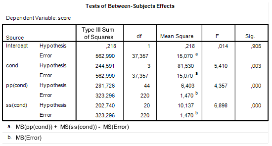
 . Let’s use the results in Figure 1 to calculate what MOE is for this particular contrast.
 , with 220 degrees of freedom and not
  , with 37.357 (see Figure 1). The consequence of this is, of course, that the 95% CI is much narrower than it should be.
 , the critical value of t is the .975 quantile of the central t distribution with
  , which equals
  . The value of MOE is therefore
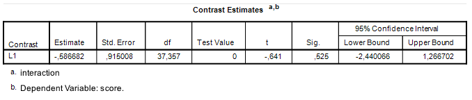
  . With a contrast estimate of
  , the 95% CI equals
 ![-0.587 \pm 0.5633 = [-1.1503, -0.0237]](https://small-s.science/wp-content/ql-cache/quicklatex.com-ea5612615f1baf096374644a223d775f_l3.png "Rendered by QuickLaTeX.com") . In comparison, using the correct value of MOE gives us
. In comparison, using the correct value of MOE gives us ![[−2.4404, 1.2664]](https://small-s.science/wp-content/ql-cache/quicklatex.com-ef97651e8790dc304790e8a8724ebed7_l3.png "Rendered by QuickLaTeX.com") .
.
 , approximate 95% CI
 ![[-1.40, 0.73]](https://small-s.science/wp-content/ql-cache/quicklatex.com-867264624a612f401b2c1cea536372a9_l3.png "Rendered by QuickLaTeX.com") , which according to the rules of thumb is a medium negative effect, but consistent with anytihing from a huge negative effect to a large positive effect in the population, as the approximate CI shows. (I have divided the point estimate and the confidence interval in Figure 2 by 1.74, to obtain Cohen’s d and an approximate confidence interval). Clearly, then, our precision can be optimized.
, which according to the rules of thumb is a medium negative effect, but consistent with anytihing from a huge negative effect to a large positive effect in the population, as the approximate CI shows. (I have divided the point estimate and the confidence interval in Figure 2 by 1.74, to obtain Cohen’s d and an approximate confidence interval). Clearly, then, our precision can be optimized. , the stimulus variance
  , and the error variance
  . Rearranging and using 1.47 as an estimate for
  . Likewise, the estimate for
  . Thus, our estimates are
  ,
,  , and
, and  .
.
 , for assurance the value .80 and the values
  , and
, and  for, respectively, Residual variance, Participant intercept variance and Stimulus intercept variance. Fill in the value 0 for all the other variances. See Figure 5.

 , to refer to the residual variance in the BwC-design, we can say
  . Normally, the precision app sums these two components to get a value for the residual variance in the BwC-design, and you will obviously get the same result if you specify the residual variance as the sum and the participant-by-stimulus variance as 0. Likewise,
  , and
, and  , where
  and
and  are the variances associated with the interaction of treatment and participant and treatment and stimulus, respectively.
 , and there is 80% assurance that MOE will not exceed
  . Note, again, that the assurance MOE is somewhat larger than target MOE, because a sample of 804 participants requires a sample of more than 500 stimuli to get the target MOE with 80% assurance and 500 stimuli is the maximum number of stimuli the app considers when minimizing the number of participants.

 ,
,  ,
,  ,
,  ,
,  , and
, and  . The Satterthwaite degrees of freedom are
  . The standard error of the contrast equals
  . The critical value for t equals
  . Expected MOE is, therefore,
  (the tiny difference with the results from the app is due to rounding errors).
 -distribution. That is, we assume with assurance
  . Now, the degrees of freedom are
  , the assurance
  , and the .80 quantile of
  . Since the relative error variance equals
  , the .80 quantile of the error variance equals
  . And this means that assurance MOE equals
  . Again, the difference with the results from the Precision App are due to rounding error.
![\[= t(df)*\sqrt{(\sum_{i=1}^a c^2_i)(\frac{1}{a}pq)^{-1}(\frac{q}{a}\sigma^2_{\alpha\beta} + \frac{p}{a}\sigma^2_{\alpha\gamma}+[\sigma^2_{\beta\gamma} + \sigma^2_e])}\]](https://small-s.science/wp-content/ql-cache/quicklatex.com-9d1fd09440d619a3e308d67a14f6d5af_l3.png "Rendered by QuickLaTeX.com")
![\[=t(df)*\sqrt{(\sum_{i=1}^a c^2_i)(pq)^{-1}(q\sigma^2_{\alpha\beta} + p\sigma^2_{\alpha\gamma}+a[\sigma^2_{\beta\gamma} + \sigma^2_e])}\]](https://small-s.science/wp-content/ql-cache/quicklatex.com-1fdcd788de0cbf5b0b33af1de00e8594_l3.png "Rendered by QuickLaTeX.com")
![\[=t(df)*\sqrt{(\sum_{i=1}^a c^2_i)(\sigma^2_{\alpha\beta}/p + \sigma^2_{\alpha\gamma}/q +a[\sigma^2_{\beta\gamma} + \sigma^2_e]/pq)}\]](https://small-s.science/wp-content/ql-cache/quicklatex.com-a6d07edd78ffac88f7f956fe4b50dcdd_l3.png "Rendered by QuickLaTeX.com")