This is an introduction to contrast analysis for estimating the linear trend among condition means with R and SPSS . The tutorial focuses on obtaining point and confidence intervals. The contents of this introduction is based on Maxwell, Delaney, and Kelley (2017) and Rosenthal, Rosnow, and Rubin (2000). I have taken the (invented) data from Haans (2018). The estimation perspective to statistical analysis is aimed at obtaining point and interval estimates of effect sizes. Here, I will use the frequentist perspective of obtaining a point estimate and a 95% Confidence Interval of the relevant effect size. For linear trend analysis, the relevant effect size is the slope coefficient of the linear trend, so, the purpose of the analysis is to estimate the value of the slope and the 95% confidence interval of the estimate. We will use contrast analysis to obtain the relevant data.
[Note: A pdf-file that differs only slightly from this blogpost can be found on my Researchgate page: here; I suggest Haans (2018) for an easy to follow introduction to contrast analysis, which should really help understanding what is being said below].
The references cited above are clear about how to construct contrast coefficients (lambda coefficients) for linear trends (and non-linear trends for that matter) that can be used to perform a significance test for the null-hypothesis that the slope equals zero. Maxwell, Delaney, and Kelley (2017) describe how to obtain a confidence interval for the slope and make clear that to obtain interpretable results from the software we use, we should consider how the linear trend contrast values are scaled. That is, standard software (like SPSS) gives us a point estimate and a confidence interval for the contrast estimate, but depending on how the coefficients are scaled, these estimates are not necessarily interpretable in terms of the slope of the linear trend, as I will make clear
momentarily.
So our goal of the data-analysis is to obtain a point and interval estimate of the slope of the linear trend and the purpose of this contribution is to show how to obtain output that is interpretable as such.
A Linear Trend
Let us have a look at an example of a linear trend to make clear what exactly we are talking about here. To keeps things simple, we suppose the following context. We have an experimental design with a single factor and a single dependent variable. The factor we are considering is quantitive and its values are equally spaced. This may (or may not) differ from the usual experiment,where the independent variable is a qualitative, nominal variable. An example from Haans (2018) is the variable location, which is the row in the lecture room where students attending the lecture are seated. There are four rows and the distance between the rows is equal. Row 1 is the row nearest to the lecturer, and row 4 is the row with the largest distance between the student and the lecturer. We will assign values 1 through 4 to the different rows.
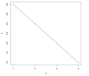
We hypothesize that the distance between the student and the lecturer, where distance is operationalized as the row where the student is seated, and mean exam scores of the students in each row show a negative linear trend. The purpose of the data-analysis is to estimate how large the (negative) slope of this linear trend is. Let us first suppose that there is a perfect negative linear trend, in the sense that each unit increase in the location variable is associated with a unit decrease in the mean exam score. Let us suppose that means are 4, 3, 2 and 1, respectively.
The negative linear trend is depicted in the following figure.
 |
| Figure 1: Negative Linear Trend with slope \beta_1 = -1.0 |
The equation for this perfect linear relation between location and mean exam score is \bar{Y} = 5 + (-1)X, that is, the slope of the negative trend equals −1. So, suppose the pattern in our sample means follows this perfect negative trend, we want our slope estimate to equal −1.
Now, following Maxwell, Delaney, and Kelley (2017), with equal sample sizes, the estimated slope of the linear trend is equal to
{\beta_1} = \frac{\hat{\psi}_{linear}}{\sum{\lambda_j^2}}, \tag{1}
which is the ratio of the linear contrast estimate
\hat{\psi} to the sum of the squared contrast weights, also called the lambda weights. (Again, for a gentle introduction to contrast analysis see
Haans (2018).) The lambda weight
\lambda_j corresponding to each value of the independent variable
Xis
\lambda_j = X_j – \bar{X}.
For the intercept of the linear trend equation we have
\hat{\beta_0} = \bar{Y} – \hat{\beta_1}\bar{X}. \tag{2}
Since the mean of the X values equals 2.5, remember that we numbered our rows 1 through 4, we have lambda weights \boldsymbol{\Lambda} = [-1.5,-0.5, 0.5, 1.5]. The value of the linear contrast estimate equals \hat{\psi} = −1.5 * 4 + −0.5 * 3 + 0.5 * 2 + 1.5 * 1 = −5 (note that this is simply the sum of the product of each lambda weight and the corresponding sample mean), the sum of the squared lambda weights equals 5, so the slope estimate equals \hat{\beta_1} = \frac{-5}{5} = -1, as it should.
The importance of scaling becomes clear if we use the standard recommended lambda weights for estimating the negative linear trend. These standard weights are \boldsymbol{\Lambda} = [-3,-1, 1, 3]. Using those weights leads to a contrast estimate of −10, and, since the sum of the squared weights now equals 20, to a slope estimate of −0.50, which is half the value we are looking for. For significance tests of the linear trend, this difference in results doesn’t matter, but for the interpretation of the slope it clearly does. Since getting the “correct” value for the slope estimate requires an additional calculation (albeit a very elementary one), I recommend sticking to setting the lambda weight to \lambda_j = X_j – \bar{X}.
Estimating the slope
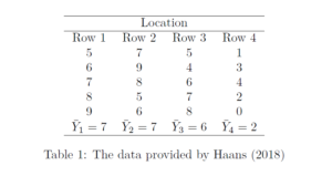
Let us apply the above to the imaginary data provided by Haans (2018) and see how we can estimate the slope of the linear trend. The data are reproduced in Table 1.
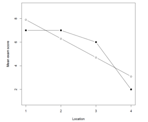
The groups means of all of the four rows are \boldsymbol{\bar{Y}} = [7, 7, 6, 2]. The lambda weights are \boldsymbol{\Lambda} = [-1.5, -0.5, 0.5, 1.5]. The value of the contrast estimate equals \hat{\psi}_{linear} = -8, the sum of the squared lambda weights equals \sum_{j=1}^{k}\lambda_{j}^{2} = 5, so the estimated slope equals -1.6. The equation for the linear trend is therefore \hat{\mu}_j = 9.5 – 1.6X_j. Figure 2 displays the obtained means and the estimated means based on the linear trend.
 |
| Figure 2: Obtained group means and estimated group means (unfilled dots) based on the linear trend. |
Obtaining the slope estimate with SPSS
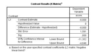
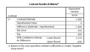
If we estimate the linear trend contrast with SPSS, we will get a point estimate of the contrast value and a 95% confidence interval estimate. For instance, if we use the lambda weights \boldsymbol{\Lambda} = [-1.5, -0.5, 0.5, 1.5] and the following syntax, we get the output presented in Figure 3. (Note: I have created a SPSS dataset with the variables row and score; see data in Table 1).
UNIANOVA score BY row
 /METHOD=SSTYPE(3)
 /INTERCEPT=INCLUDE
 /CRITERIA=ALPHA(0.05)
 /LMATRIX = "Negative linear trend?"
   row -1.5 -0.5 0.5 1.5 intercept 0
/DESIGN=row.
 |
| Figure 3: SPSS Output Linear Trend Contrast |
Figure 3 makes it clear that the 95% CI is of the linear trend contrast estimate, and not of the slope. But it is easy to obtain a confidence interval for the slope estimate by using (1) on the limits of the CI of the contrast estimate. Since the sum of the squared lambda weights equals 5.0, the confidence interval for the slope estimate is 95% CI [-11.352/5, -4.648/5] = [-2.27, -0.93]. Alternatively, divide the lambda weights by the sum of the squared lambda weights and use the results in the specification of the L-matrix in SPSS:
UNIANOVA score BY row
 /METHOD=SSTYPE(3)
 /INTERCEPT=INCLUDE
 /CRITERIA=ALPHA(0.05)
 /LMATRIX = "Negative linear trend?"
   row -1.5/5 -0.5/5 0.5/5 1.5/5 intercept 0
/DESIGN=row.
Using the syntax above leads to the results presented in Figure 4.
 |
| Figure 4: SPSS Output Slope Estimate with adjusted contrast weights |
Obtaining the estimation results with R
The following R-code accomplishes the same goals. (Note: I make use of the emmeans package, so you need to install that package first; I have created an RData-file named betweenData.Rdata using the data in Table 1, using the variable names location and examscore).
# load the dataset

load('~\betweenData.RData')

# load the functions of the emmeans package
library(emmeans)

# set options for the emmeans package to get
# only confidence intervals set infer=c(TRUE, TRUE)for both
# CI and p-value

emm_options(contrast = list(infer=c(TRUE, FALSE)))


# specify the contrast (note divide
# by sum of squared contrast weights)

myContrast = c(-1.5, -0.5, 0.5, 1.5)/ 5

# fit the model (this assumes the data are
# available in the workspace)

theMod = lm(examscore ~ location)

# get expected marginal means
theMeans = emmeans(theMod, "location")

contrast(theMeans, list("Slope"=myContrast))
##  contrast estimate        SE df  lower.CL   upper.CL
##  Slope        -1.6 0.3162278 16 -2.270373 -0.9296271
##
## Confidence level used: 0.95
Interpreting the results
The estimate of the slope of the linear trend equals \hat{\beta}_1 = -1.60, 95% CI [-2.27, -0.93]. This means that with each increase in row number (from a given row to a location one row further away from the lecturer) the estimated exam score will on average decrease by -1.6 points, but any value between -2.27 and -0.93 is considered to be a relatively plausible candidate value, with 95% confidence. (Of course, we should probably not extrapolate beyond the rows that were actually observed, otherwise students seated behind the lecturer will be expected to have a higher population mean than students seated in front of the lecturer).
In order to aid interpretation one may convert these numbers to a standardized version (resulting in the standardized confidence interval of the slope estimate) and use rules-of-thumb for interpretation. The square root of the within condition variance may be a suitable standardizer. The value of this standardizer is S_{W} = 1.58 (I obtained the value of \text{MS}_{within} = 2.5 from the SPSS ANOVA table). The standardized estimates are therefore -1.0, 95% CI [-1.43, -0.59] suggesting that the negative effect of moving one row further from the lecturer is somewhere between medium and very large, with the point estimate corresponding to a large negative effect.
References
Maxwell, S.E., Delaney, H. D., & Kelley, K. (2017). Designing Experiments and Analyzing Data. A Model Comparison Perspective. (Third Edition). New York/ London: Routledge.
Rosenthal, R., Rosnow, R.L., & Rubin, D.B. (1993). Contrasts and Effect Sizes in Behavioral Research. A Correlational Approach. Cambridge, UK: Cambridge University Press.
