Planning for precision requires that we choose a target Margin of Error (MoE; see this post for an introduction to the basic concepts) and a value for assurance, the probability that MoE will not exceed our target MoE. What your exact target MoE will be depends on your research goals, of course.
Cumming and Calin-Jageman (2017, p. 277) propose a strategy for determining target MoE. You can use this strategy if your research goal is to provide strong evidence that the effect size is non-zero. The strategy is to divide the expected value of the difference by two, and to use that result as your target MoE.
Let’s restrict our attention to the comparison of two means. If the expected difference between the two means is Cohens’s d = .80, the proposed strategy is to set your target MoE at f = .40, which means that your target MoE is set at .40 standard deviations. If you plan for this value of target MoE with 80% assurance, the recommended sample size is n = 55 participants per group. These results are guaranteed to be true, if it is known for a fact that Cohen’s d is .80 and all statistical assumptions apply.
But it is generally not known for a fact that Cohen’s d has a particular value and so we need to answer a non-trivial question: what effect size can we reasonably expect? And, how can we have assurance that the MoE will not exceed half the unknown true effect size? One of the many options we have for answering this question is to conduct a pilot study, estimate the plausible values of the effect size and use these values for sample size planning. I will describe a strategy that basically mirrors the sample size planning for power approach described by Anderson, Kelley, and Maxwell (2017).
The procedure is as follows. In order to plan with approximately 80% assurance, estimate on the basis of your pilot the 80% confidence interval for the population effect size and use half the value of the lower limit for sample size planning with 90% assurance. This will give you 81% assurance that assurance MoE is no larger than half the unknown true effect size.
The logic of planning with assurance, with assurance
There are two “problems” we need to consider when estimating the true effect size. The first problem is that there is at least 50% probability of obtaining an overestimate of the true effect size. If that happens, and we take the point estimate of the effect size as input for sample size planning, what we “believe” to be a sample size sufficient for 80% assurance will be a sample size that has less than 80% assurance at least 50% of the times. So, using the point estimate gives assurance MoE for the unknown effect size with less than 50% assurance.
To make it more concrete: suppose the true effect equals .80, and we use n = 25 participants in both groups of the pilot study, the probability is approximately 50% that the point estimate is above .80. This implies, of course, that we will plan for a value of f > .40, approximately 50% of the times, and so the sample we get will only give us 80% assurance 50% of the times.
The second problem is that the small sample sizes we normally use for pilot studies may give highly imprecise estimates. For instance, with n = 25 participants per group, the expected MoE is f = 0.5687. So, even if we accept 50% assurance, it is highly likely that the point estimate is rather imprecise.
Since we are considering a pilot study, one of the obvious solutions, increasing the sample size so that expected MoE is likely to be small, is not really an option. But what we can do is to use an estimate that is unlikely to be an overestimate of the true effect size. In particular, we can use as our estimate the lower limit of a confidence interval for the effect size.
Let me explain, by considering the 80% CI of the effect size estimate. From basic theory it follows that the “true” value of the effect size will be smaller than the lower limit of the 80% confidence interval with probability equal to 10%. That is, if we calculate a huge number of 80% confidence intervals, each time on the basis of new random samples from the population, the true value of the effect size will be below the lower limit in 10% of the cases. This also means that the lower limit of the interval has 90% probability to not overestimate the true effect size.
This means that if we take the lower limit of the 80% CI of the pilot estimate as input for our sample size calculations, and if we plan with assurance of .90, we will have 90%*90% = 81% assurance that using the sample size we get from our calculations will have MoE no larger than half the true effect size. (Note that for 80% CI’s with negative limits you should choose the upper limit).
Sample Size planning based on a pilot study
Student of mine recently did a pilot study. This was a pilot for an experiment investigating the size of the effect of fluency of delivery of a spoken message in a video on Comprehensibility, Persuasiveness and viewers’ Appreciation of the video. The pilot study used two groups of size n = 10, one group watched the fluent video (without ‘eh’) and the other group watched the disfluent video where the speaker used ‘eh’ a lot. The dependent variables were measured on 7-point scales.
Let’s look at the results for the Appreciation variable. The (biased) estimate of Cohen’s d (based on the pooled standard deviation) equals 1.09, 80% CI [0.46, 1.69] (I’ve calculated this using the ci.smd function from the MBESS-package. According to the rules-of-thumb for interpreting Cohen’s d, this can be considered a large effect. (For communication effect studies it can be considered an insanely large effect). However, the CI shows the large imprecision of the result, which is of course what we can expect with sample sizes of n = 10. (Average MoE equals f = 0.95, and according to my rules-of-thumb that is well below what I consider to be borderline precise).
If we use the lower limit of the interval (d = 0.46), sample size planning with 90% assurance for half that effect (f = 0.23) gives us a sample size equal to n = 162. (Technical note: I planned for the half-width of the standardized CI of the unstandardized effect size, not for the CI of the standardized effect size; I used my Shiny App for planning assuming an independent groups design with two groups). As explained, since we used the lower limit of the 80% CI of the pilot and used 90% assurance in planning the sample size, the assurance that MoE will not exceed half the unknown true effect size equals 81%.


 of the simple linear regression equation
  . The basic ingredients we need for sample size planning are a measure of the precision, a way to determine the quantiles of the sampling distribution of our measure of precision, and a way to calculate sample sizes.
 , where
  , is the .975 quantile of the central t-distribution with
  degrees of freedom, and
  is the standard error of the estimate of
  (Wilcox, 2017): the variance of Y given X divided by the sum of squared errors of X. The variance
  equals
  , the variance of Y multiplied by 1 minus the squared population correlation between Y and X, and it is estimated with the residual variance
  , where
  .
.![\[\hat{\sigma}_{\hat{\beta_{1}}}^{2}=\frac{\sum(Y-\hat{Y})^{2}/df_{e}}{\sum(X-\bar{X})^{2}}. \]](https://small-s.science/wp-content/ql-cache/quicklatex.com-712f2857df79a9cc19ad5198431f2877_l3.png "Rendered by QuickLaTeX.com")
 -distribution:
![\[\frac{\sum(Y-\hat{Y})^{2}}{\sigma_{y}^{2}(1-\rho^{2})}\sim\chi^{2}(df_{e}),\]](https://small-s.science/wp-content/ql-cache/quicklatex.com-5fb82f0623b2088e7771fbf7e7d4803c_l3.png "Rendered by QuickLaTeX.com")
![\[\frac{\sum(Y-\hat{Y})^{2}}{df_{e}}\sim\frac{\sigma_{y}^{2}(1-\rho^{2})\chi^{2}(df_{e})}{df_{e}}.\]](https://small-s.science/wp-content/ql-cache/quicklatex.com-6f1e262a579b65243e1854e59a4243d6_l3.png "Rendered by QuickLaTeX.com")
![\[\frac{\sum(X-\bar{X})^{2}}{\sigma_{X}^{2}}\sim\chi^{2}(df),\]](https://small-s.science/wp-content/ql-cache/quicklatex.com-fe2f47a4c99a2963559b96659fb59616_l3.png "Rendered by QuickLaTeX.com")
 , therefore
![\[\sum(X-\bar{X})^{2}\sim\sigma_{X}^{2}\chi^{2}(df).\]](https://small-s.science/wp-content/ql-cache/quicklatex.com-e793ae0023912bb5ee2c4d42856eb6a8_l3.png "Rendered by QuickLaTeX.com")
 , and multiplying by 1 (
 ).
).![\[df\sigma_{X}^{2}\sim df\sigma_{X}^{2}\chi^{2}(df)/df.\]](https://small-s.science/wp-content/ql-cache/quicklatex.com-0f86831fd6d9113dcff83251b70eb992_l3.png "Rendered by QuickLaTeX.com")
![\[\hat{\sigma}_{\hat{\beta_{1}}}^{2}\sim\frac{\sigma_{y}^{2}(1-\rho^{2})\chi^{2}(df_{e})/df_{e}}{df\sigma_{X}^{2}\chi^{2}(df)/df}=\frac{\sigma_{y}^{2}(1-\rho^{2})}{df\sigma_{X}^{2}}\frac{\chi^{2}(df_{e})/df_{e}}{\chi^{2}(df)/df}=\frac{\sigma_{y}^{2}(1-\rho^{2})F(df_{e,}df)}{df\sigma_{X}^{2}},\]](https://small-s.science/wp-content/ql-cache/quicklatex.com-cdc57f8bf40a827845ec2f30dcfb8751_l3.png "Rendered by QuickLaTeX.com")
![\[\hat{MOE}\sim t_{.975}(N-2)\sqrt{\frac{\sigma_{y}^{2}(1-\rho^{2})F(N-2,N-1)}{(N-1)\sigma_{X}^{2}}}. \]](https://small-s.science/wp-content/ql-cache/quicklatex.com-f0b396b6b94f61a97099bec31546363b_l3.png "Rendered by QuickLaTeX.com")
 ,
,  ,
,  ,
,  , and assurance is .80, then according to (2), 80% of estimated MOEs will not exceed the value given by:
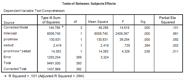
![\[\hat{\sigma_\psi}= \sqrt{\sum{c_i^2MS_e/n_i}},\]](https://small-s.science/wp-content/ql-cache/quicklatex.com-e711016f1b800409ee4d1632159091d7_l3.png "Rendered by QuickLaTeX.com")
 is the contrast weight for the i-th condition mean, and
  the number of observations (in our example participants) in treatment condition i. Note that
  is the variance of treatment mean i, the square root of which gives the familiar standard error of the mean.
![\[MOE = t_{.975}(df_e)\sqrt{\sum{c_i^2MS_e/n_i}}=t_{.975}(df_e)\sqrt{4MS_e/n_i} = 2t_{.975}(df_e)\sqrt{MS_e/n_i}.\]](https://small-s.science/wp-content/ql-cache/quicklatex.com-c566353662177824c69974b4d59785d4_l3.png "Rendered by QuickLaTeX.com")
 , and the true value of Mean Square Error is 3.324, then MOE for the contrast estimate equals
![\[MOE = 2*t_{.975}(396)*\sqrt{3.324/100} = 0.7071\]](https://small-s.science/wp-content/ql-cache/quicklatex.com-98e408fbb1899034420a41dc86f58115_l3.png "Rendered by QuickLaTeX.com")
![\[MOE = 2*t_{.975}(df_e)\sqrt{(MS_w / n_i)},\]](https://small-s.science/wp-content/ql-cache/quicklatex.com-1984a751953fc6b0698d72e7bf2c550b_l3.png "Rendered by QuickLaTeX.com")
 , since we are considering the 2×2 design.
![\[0.4558 = 2*t_{.975}(4(n_i - 1)\sqrt{(MS_w / n_i)},\]](https://small-s.science/wp-content/ql-cache/quicklatex.com-9a775e47b691309421ea2f9d94c016c2_l3.png "Rendered by QuickLaTeX.com")
![\[MOE_{\gamma} = 2*t_{.975}(df)*\sqrt{MS_w/n_i*\chi^2_{\gamma}(df)/df},\]](https://small-s.science/wp-content/ql-cache/quicklatex.com-f5945fe8ef0dad8f2bf28d70a7553fae_l3.png "Rendered by QuickLaTeX.com")
 is the assurance expressed in a probability between 0 and 1.


 we have the following expression for the expected MOE.
 ![\[E(MOE) = t_{.975}(df)*\sigma_{\hat{\psi}},\]](https://small-s.science/wp-content/ql-cache/quicklatex.com-3c365ea8bf332e7cfe0131922eaadfca_l3.png "Rendered by QuickLaTeX.com")
 is the standard error of the contrast estimate. Of course, both the standard error and the df are functions of the sample sizes.
 , where a is the number of treatment conditions, we use the following general expression.
![\[\sigma_{\hat{\psi}} = \sqrt{\sum c^2_i \frac{\sigma^2_w}{n}},\]](https://small-s.science/wp-content/ql-cache/quicklatex.com-2047baef6bfe75fa33fdb76808ad99fe_l3.png "Rendered by QuickLaTeX.com")
 the within treatment variance (we assume homogeneity of variance).
 and
and  , and
, and  , the standard error for this contrast equals
  . (Note that this is simply the standard error of the difference between two means as used in the independent samples t-test).
 . The expected MOE for this design is therefore,
  . Note that using these figures entails that 95% of the contrast estimates will take values between the true contrast value plus and minus the expected MOE:
  .
. }, the same sample sizes and within treatment variance gives
  .
.![\[MS_w \sim \sigma^2_w*\chi^2(df)/df,\]](https://small-s.science/wp-content/ql-cache/quicklatex.com-33d9394fa378a467d81b18b1eebf8d8d_l3.png "Rendered by QuickLaTeX.com")
![\[\hat{MOE} \sim t_{.975}(df)\sqrt{\frac{1}{n}\sum{c_i^2}\sigma^2_w*\chi^2(df)/df}.\]](https://small-s.science/wp-content/ql-cache/quicklatex.com-55d2923233b4c1800935a900bed6c86c_l3.png "Rendered by QuickLaTeX.com")
![\[\hat{MOE}_{.80} = 2.0244 * \sqrt{1/20*2*20*45.07628/38} = 3.1181.\]](https://small-s.science/wp-content/ql-cache/quicklatex.com-7389e9cdfe17c1809754f3a5cdf0962f_l3.png "Rendered by QuickLaTeX.com")
 in the chi-squared (df = 38) distribution. That is
  .
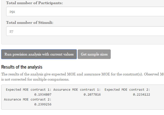
. ) and will find the combination of number of participants and items that will give an estimated MOE no larger than target MOE in
  , and the number of observations in each group by list combination equals
  . The condition means are estimated by combining a group by list combinations each of which composed of different participants and stimuli. The total number of observations per condition is therefore,
  .
.![\[Y_{ijk} = \mu + \alpha_i + \beta_j + \gamma_k + (\alpha\beta)_{ij} + (\alpha\gamma)_{ik} + e_{ijk},\]](https://small-s.science/wp-content/ql-cache/quicklatex.com-0fe0fded4cedc1ede78c9f5dcd9c1c61_l3.png "Rendered by QuickLaTeX.com")
 is a constant treatment effect (it’s a fixed effect), and the other effect are random effects with zero mean and variances
  (participants),
  (items),
  (person by treatment interaction),
  (item by treatment interaction) and
  (error variance confounded with the person by item interaction). Note: in Table 1 below,
 ![[\sigma^2_{\beta\gamma} + \sigma^2_e]](https://small-s.science/wp-content/ql-cache/quicklatex.com-04ba4ecdae4334a2a41e0f4ab3c241f2_l3.png "Rendered by QuickLaTeX.com") .
. , and
, and  . The latter two restrictions make the interaction-effects correlated across conditions (i,e. the effects of person and treatment are correlated across condition for the same person, likewise the interaction effects of item and treatment are correlated across conditons for the same item. Interaction effects of different participants and items are uncorrelated). The covariances between the random effects
  are assumed to be zero.
 , and
, and  . Furthermore, the covariance of the interactions between treatment and participant or between treatment and item for the same participant or item are
  for participants and
  for items.
 ). Thus,
 ![\sigma^2_w = \frac{q}{a}\sigma^2_{\alpha\beta} + \frac{p}{a}\sigma^2_{\alpha\gamma}+[\sigma^2_{\beta\gamma} + \sigma^2_e]](https://small-s.science/wp-content/ql-cache/quicklatex.com-6a8143341552d56735cb6827e1d9d309_l3.png "Rendered by QuickLaTeX.com") . Note that the latter equals the sum of the expected mean squares of the Treatment by Participant (
. Note that the latter equals the sum of the expected mean squares of the Treatment by Participant ( ) and the Treatment by Item (
 ) interactions, minus the expected mean square associated with Error (
 ).
).![\[df =\frac{(E(MS_{tp}) + E(MS_{ti}) - E(MS_e))^2}{\frac{E(MS_{tp})^2}{(a - 1)(p-a)}+\frac{E(MS_{ti})^2}{(a - 1)(q-a)}+\frac{E(MS_e)^2}{(p-a)(q-a)}}\]](https://small-s.science/wp-content/ql-cache/quicklatex.com-9d20ad417c928f844eff686d67e11de2_l3.png "Rendered by QuickLaTeX.com")
![\[E(MOE) = t(df)*\sqrt{(\sum_{i=1}^a c^2_i)(\frac{1}{a}pq)^{-1}\sigma^2_w}\]](https://small-s.science/wp-content/ql-cache/quicklatex.com-c0d601b03e80c69eaa13d78d5fa26d94_l3.png "Rendered by QuickLaTeX.com")
![\[= t(df)*\sqrt{(\sum_{i=1}^a c^2_i)(\frac{1}{a}pq)^{-1}(\frac{q}{a}\sigma^2_{\alpha\beta} + \frac{p}{a}\sigma^2_{\alpha\gamma}+[\sigma^2_{\beta\gamma} + \sigma^2_e])}\]](https://small-s.science/wp-content/ql-cache/quicklatex.com-9d1fd09440d619a3e308d67a14f6d5af_l3.png "Rendered by QuickLaTeX.com")
![\[=t(df)*\sqrt{(\sum_{i=1}^a c^2_i)(pq)^{-1}(q\sigma^2_{\alpha\beta} + p\sigma^2_{\alpha\gamma}+a[\sigma^2_{\beta\gamma} + \sigma^2_e])}\]](https://small-s.science/wp-content/ql-cache/quicklatex.com-1fdcd788de0cbf5b0b33af1de00e8594_l3.png "Rendered by QuickLaTeX.com")
![\[=t(df)*\sqrt{(\sum_{i=1}^a c^2_i)(\sigma^2_{\alpha\beta}/p + \sigma^2_{\alpha\gamma}/q +a[\sigma^2_{\beta\gamma} + \sigma^2_e]/pq)}\]](https://small-s.science/wp-content/ql-cache/quicklatex.com-a6d07edd78ffac88f7f956fe4b50dcdd_l3.png "Rendered by QuickLaTeX.com")
 . Suppose furthermore, that 10% of the variance can be attributed to treatment by participant interaction, 10% of the variance to the treatment by item interaction and 40% of the variance to the error confounded with the participant by item interaction. (which leaves 40% of the total variance attributable to participant and item variance.
 ,
,  , and
, and  . Our target MOE is .25, and we plan to use the counterbalanced design with p = 30 participants, and q = 15 items (stimuli).
 ,
,  , and
, and  , and the approximate df equal
  .
. .
.