In this post, I want to show how to do contrast analysis with R for factorial designs. We focus on a 2-way between subjects design. A tutorial for factorial within-subjects designs can be found here: https://small-s.science/2019/01/contrast-analysis-with-r-repeated-measures/ . A tutorial for mixed designs (combining within and between subjects factors can be found here: https://small-s.science/2019/04/contrast-analysis-with-r-mixed-design/.
I want to show how we can use R for contrast analysis of an interaction effect in a 2 x 4 between subjects design. The analysis onsiders the effect of students’ seating distance from the teacher and the educational performance of the students: the closer to the teacher the student is seated, the higher the performance. A “theory “explaining the effect is that the effect is mainly caused by the teacher having decreased levels of eye contact with the students sitting farther to the back in the lecture hall.
To test that theory, a experiment was conducted with N = 72 participants attending a lecture. The lecture was given to two independent groups of 36 participants. The first group attended the lecture while the teacher was wearing dark sunglasses, the second group attented the lecture while the teacher was not wearing sunglasses. All participants were randomly assigned to 1 of 4 possible rows, with row 1 being closest to the teacher and row 4 the furthest from the teacher The dependent variable was the score on a 10-item questionnaire about the contents of the lecture. So, we have a 2 by 4 factorial design, with n = 9 participants in each combination of the factor levels.
Here we focus on obtaining an interaction contrast: we will estimate the extent to which the difference between the mean retention score of the participants on the first row and those on the other rows differs between the conditions with and without sunglasses.
The interaction contrast with SPSS
I’ve downloaded a dataset from the supplementary materials accompanying Haans (2018) from http://pareonline.net/sup/v23n9.zip (Between2by4data.sav) and I ran the following syntax in SPSS:
UNIANOVA retention BY sunglasses location
 /LMATRIX = "Interaction contrast"
  sunglasses*location 1 -1/3 -1/3 -1/3 -1 1/3 1/3 1/3 intercept 0
   /DESIGN= sunglasses*location.
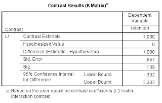
Table 1 is the relevant part of the output.
So, the estimate of the interaction contrasts equals 1.00, 95% CI [-0.332, 2.332]. (See this post for optimizing the sample size to get a more precise estimate than this).
Contrast analysis with R for factorial designs
Let’s see how we can get the same results with R.
library(MASS)
library(foreign)

theData <- read.spss("./Between2by4data.sav")
theData <- as.data.frame(theData)

attach(theData)

# setting contrasts
contrasts(sunglasses) <- ginv(rbind(c(1, -1)))
contrasts(location)  <- ginv(rbind(c(1, -1/3, -1/3, -1/3),
                                   c(0, 1, -1/2, -1/2), c(0, 0, 1, -1)))

# fitting model

myMod <- lm(retention ~ sunglasses*location)
The code above achieves the following. First the relevant packages are loaded. The MASS package provides the function ginv, which we need to specify custom contrasts and the Foreign package contains the function read.spss, which enables R to read SPSS .sav datafiles.
Getting custom contrast estimates involves calculating the generalized inverse of the contrast matrices for the two factors. Each contrast is specified on the rows of these contrast matrices. For instance, the contrast matrix for the factor location, which has 4 levels, consists of 3 rows and 4 columns. In the above code, the matrix is specified with the function rbind, which basically says that the three contrast weight vectors c(1, -1/3, -1/3, -1/3), c(0, 1, -1/2, -1/2), c(0, 0, 1, -1) form the three rows of the contrast matrix that we use as an argument of the ginv function. (Note that the set of contrasts consists of orthogonal Helmert contrasts).
The last call is our call to the lm-function which estimates the contrasts. Let’s have a look at these estimates.
summary(myMod)
##
## Call:
## lm(formula = retention ~ sunglasses * location)
##
## Residuals:
##    Min     1Q Median     3Q    Max
##     -2     -1      0      1      2
##
## Coefficients:
##                       Estimate Std. Error t value Pr(>|t|)
## (Intercept)             5.3750     0.1443  37.239  < 2e-16 ***
## sunglasses1             1.2500     0.2887   4.330 5.35e-05 ***
## location1               2.1667     0.3333   6.500 1.39e-08 ***
## location2               1.0000     0.3536   2.828  0.00624 **
## location3               2.0000     0.4082   4.899 6.88e-06 ***
## sunglasses1:location1   1.0000     0.6667   1.500  0.13853
## sunglasses1:location2   3.0000     0.7071   4.243 7.26e-05 ***
## sunglasses1:location3   2.0000     0.8165   2.449  0.01705 *
## ---
## Signif. codes:  0 '***' 0.001 '**' 0.01 '*' 0.05 '.' 0.1 ' ' 1
##
## Residual standard error: 1.225 on 64 degrees of freedom
## Multiple R-squared:  0.6508, Adjusted R-squared:  0.6126
## F-statistic: 17.04 on 7 and 64 DF,  p-value: 1.7e-12
For the present purposes, we will consider the estimate of the first interaction contrast, which estimates the difference between the means of the first and the other rows between the with and without sunglasses conditions. So, we will have to look at the sunglasses1:location1 row of the output.
Unsurprisingly, the estimate of the contrast and its standard error are the same as in the SPSS ouput in Table 1. The estimate equals 1.00 and the standard error equals 0.6667.
Note that the residual degrees of freedom equal 64. This is equal to the product of the number of levels of each factor, 2 and 4, and the number of participants (9) per combination of the levels minus 1: df = 2*4*(9 – 1) = 64. We will use these degrees of freedom to obtain a confidence interval of the estimate.
We will calculate the confidence interval by first extracting the contrast estimate and the standard error, after which we multiply the standard error by the critical value of t with df = 64 and add the result to and substract it from the contrast estimate:
estimate = myMod$coefficients["sunglasses1:location1"]

se = sqrt(diag(vcov(myMod)))["sunglasses1:location1"]

df = 2*4*(9 - 1)

# confidence interval

estimate + c(-qt(.975, df), qt(.975, df))*se
## [1] -0.3318198 2.3318198
Clearly, we have replicated all the estimation results presented in Table 1.
Reference
Haans, Antal (2018). Contrast Analysis: A Tutorial. Practical Assessment, Research, & Education, 23(9). Available online: http://pareonline.net/getvn.asp?v=23&n=9

