This is a tutorial for a planning for precision of contrasts estimates. The application is here: https://gmulder.shinyapps.io/PlanningContrasts/.
NOTE: For a (beta) version of planning for factoral designs: http://small-s.science/?p=18
NOTE: I’ve updated the app with a few corrections, so there is a new version. (The November version has corrected degrees of freedom for the 3 and 4 condition within design).
If you like to run the app in R, install the shiny and devtool packages and run the following:
library(shiny)
library(devtools)
source_url("https://git.io/fpI1R")
shinyApp(ui = ui, server = server)
Specifying Target MoE and Assurance
| Description | f |
|---|---|
| Extremely Precise | .05 |
| Very Precise | .10 |
| Precise | .25 |
| Reasonably Precise | .40 |
| Borderline Precise | .65 |
Specifying the Design
Specifying the Cross-Condition correlation
Note: for technical reasons a correlation of 1 will be automatically changed to .99.
For independent designs the correlation should equal 0. (And the above story about reliability does no longer make sense; but we also do not need it).
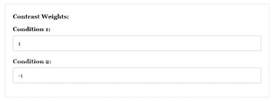
Specifying Contrasts
Contrasts must obey the following rules.
- The sum of the contrast weights must equal zero;
- The sum of the absolute values of the contrast must be equal to two.
Examples
 |
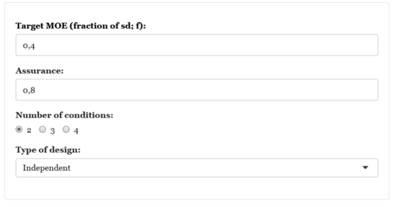
| Figure 1. Values for Target MoE, assurance and design |
 |
| Figure 2: Standard contrasts for comparison of two conditions |
The output is as follows:
The results give you the sample size for each condition (n), and information about target MoE (f), assurance (assu), the number of conditions (k), and the cross-condition correlation (cor; the value is zero, as it should be in the independent design). With n = 55, there is a 80% probability that f will not be larger than .40.
If you use 55 participants per group the expected MoE equals 0.38.
Of course, using 55 participants per group, makes the total sample size equal to 110.
The output also included a plot of the expected results (what you can expect to happen on average). See Figure 3.
 |
| Figure 3: Expected results using n = 55 participants per group in the two groups independent design |
This output helps you to consider whether the Expected MoE is small enough. Suppose, for instance, that true difference equals .5 standard deviations, i.e. a medium effect. The figure shows that the expected contrast estimate is a medium effect, and the confidence interval shows that on average values ranging from small to large effects [.12, .88] will be included in the interval. If the difference between small, medium and large effects is important, an expected precision of f = .38 may not be enough, although small and large effects are at the limits of the confidence interval.
A four groups dependent design
Technical Note: The app assumes that the sum of squares of the Error Variance can be decomposed in (k – 1) equal parts, where k is the number of conditions. I will change this restriction in a future version of the app. For a custom contrast it is assumed that the contrast is part of an orthogonal set.
Suppose your major interest is the comparison between the average of two groups and the average of two other groups. You have a dependent (repeated measures) design in which participants will be exposed to each of the four treatment conditions. Let’s plan for a target MoE of f = 0.25, with 80 % assurance and let’s suppose our cross-condition correlation equals r = .70. I choose a custom contrast with weights {1/2, 1/2, -1/2, -1/2} (see Figure 4).
 |
| Figure 4. Input for sample size planning |
The output is as follows.
So, we need 26 participants to have 80% assurance that obtained MoE will not be larger than f = 0.25. Expected MoE is equal to .22. According to the guidelines above, this is a precise estimate.
If you choose “Helmert Contrasts” instead, and press the button without changing anything, the output is as follows.
Under Expected Moe you will see for each of the three contrasts c1, c2, and c3, the weights and expected MOE. The 46 participants give an expected MoE smaller than target MoE, for the least precise estimate (c3; the pairwise comparison) the other expected MoE’s are smaller than that. The Expected Results Figure will display the results for the contrasts with the largest expected MoE.


