Contrast Analysis for Within Subjects Designs with R: a Tutorial.

In this post, I illustrate how to do contrast analysis for within subjects designs with  R.  A within subjects design is also called a repeated measures design.  I will illustrate two approaches. The first is to simply use the one-sample t-test on the transformed scores. This will replicate a contrast analysis done with SPSS GLM Repeated Measures. The second is to make use of mixed linear effects modeling with the lmer-function from the lme4 library.

Conceptually, the major difference between the two approaches is that in the latter approach we make use of a single shared error variance and covariance across conditions (we assume compound symmetry), whereas in the former each contrast has a separate error variance, depending on the specific conditions involved in the contrast (these conditions may have unequal variances and covariances).

As in the previous post (https://small-s.science/2018/12/contrast-analysis-with-r-tutorial/), we will focus our attention on obtaining an interaction contrast estimate.

Again, our example is taken from Haans (2018; see also this post). It considers the effect of students’ seating distance from the teacher and the educational performance of the students: the closer to the teacher the student is seated, the higher the performance. A “theory “explaining the effect is that the effect is mainly caused by the teacher having decreased levels of eye contact with the students sitting farther to the back in the lecture hall.

To test that theory, a experiment was conducted with N = 9 participants in a completely within-subjects-design (also called a fully-crossed design), with two fixed factors: sunglasses (with or without) and location (row 1 through row 4). The dependent variable was the score on a 10-item questionnaire about the contents of the lecture. So, we have a 2 by 4 within-subjects-design, with n = 9 participants in each combination of the factor levels.

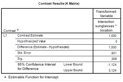
We will again focus on obtaining an interaction contrast: we will estimate the extent to which the difference between the mean retention score on the first row and those on the other rows differs between the conditions with and without sunglasses.

Contrast Analysis with SPSS Repeated Measures

Continue reading “Contrast Analysis for Within Subjects Designs with R: a Tutorial.”

Custom contrasts for the one-way repeated measures design using Lmer

Here is some code for doing one-way repeated measures analysis with lme4 and custom contrasts. We will use a repeated measures design with three conditions of the factor Treat and 20 participants. The contrasts are Helmert contrasts, but they differ from the built-in Helmert contrasts in that the sum of the absolute values of the contrasts weights equals 2 for each contrast.
The standard error of each contrast equals the square root of the product of the sum of the squared contrast weight w and the residual variance divided by the number of participants n.

    \[\sigma_{\hat{\psi}} =  \sqrt{\sum{w_i}\sigma^2_e/n}\]

The residual variance equals the within treatment variance times 1 minus the correlation between conditions. (Which equals the within treatment variance minus 1 times the covariance \rho\sigma^2_{within}) .

    \[\sigma^2_e = \sigma^2_{within}(1 - \rho)\]

In the example below, the within treatment variance equals 1 and the covariance 0.5 (so the value of the correlation is .50 as well). The residual variance is therefore equal to .50.

For the first contrasts, the weights are equal to {-1, 1, 0}, so the value of the standard error of the contrasts should be equal to the square root of 2*.50/20 = 0.2236.

library(MASS)
library(lme4)
# setting up treatment and participants factors
nTreat = 3
nPP = 20
Treat <- factor(rep(1:nTreat, each=nPP))
PP <- factor(rep(1:nPP, nTreat))

# generate some random 
# specify means

means = c(0, .20, .50)

# create variance-covariance matrix
# var = 1, cov = .5
Sigma = matrix(rep(.5, 9), 3, 3)
diag(Sigma) <- 1

# generate the data; using empirical = TRUE
# so that variance and covariance are known
# set to FALSE for "real" random data

sco = as.vector(mvrnorm(nPP, means, Sigma, empirical = TRUE))

#setting up custom contrasts for Treatment factor 
myContrasts <- rbind(c(-1, 1, 0), c(-.5, -.5, 1))
contrasts(Treat) <- ginv(myContrasts)

#fit linear mixed effects model: 
myModel <- lmer(sco ~ Treat + (1|PP))

summary(myModel)
## Linear mixed model fit by REML ['lmerMod']
## Formula: sco ~ Treat + (1 | PP)
## 
## REML criterion at convergence: 157.6
## 
## Scaled residuals: 
##     Min      1Q  Median      3Q     Max 
## -2.6676 -0.4869  0.1056  0.6053  1.9529 
## 
## Random effects:
##  Groups   Name        Variance Std.Dev.
##  PP       (Intercept) 0.5      0.7071  
##  Residual             0.5      0.7071  
## Number of obs: 60, groups:  PP, 20
## 
## Fixed effects:
##             Estimate Std. Error t value
## (Intercept)   0.2333     0.1826   1.278
## Treat1        0.2000     0.2236   0.894
## Treat2        0.4000     0.1936   2.066
## 
## Correlation of Fixed Effects:
##        (Intr) Treat1
## Treat1 0.000        
## Treat2 0.000  0.000