Planning for precise contrasts in two-way factorial designs: a Tutorial

I’ve created a first version of Shiny App for sample size planning for precise contrast estimates in one and two-way designs. So, if you want to plan for interaction contrasts for two-way designs, take a look here: https://gmulder.shinyapps.io/PlanningFactorialContrasts/

Important: this is a first version that contains no error checking (but you know what you’re doing, so that’s not a problem). Also, I have not tested the results of the app with simulation studies. As soon as I have done that, I will share the code of the app.

Update: The values for the factorial two-way within subjects designs are checked with simulation studies (for f = .40, assurance = .80, and correlation rho = .50).

Note: if you have a single factor design, you may also consider looking here: http://small-s.science/?p=19

Note: if you have a two-groups independent design, go here for an introduction to sample size planning and its relation to the power of the t-test: http://small-s.science/?p=25

See for more detailed information about sample size planning for single factor and factorial designs (between, within, and mixed): http://small-s.science/?p=10 and for guidelines for setting target MoE: http://small-s.science/?p=14)

How does the app work?

1. Specifying Target MoE and Assurance 

Target MoE should be specified in a number of standard deviations (usually a fraction; for details see Cumming, 2012; Cumming & Calin-Jageman, 2017). The symbol f will be used to refer to this standardized MoE. Target MoE (f) must be larger than zero (f will be automatically set to .05 if you accidentally fill in the value 0). 
I suggest using the following guidelines for target MoE (f): 
Description f
Extremely Precise .05
Very Precise .10
Precise .25
Reasonably Precise .40
Borderline Precise .65
You should only use these guidelines if you lack the information you need for specifying a reasonable value for Target MoE.

Assurance is the probability that (to be) obtained MoE will be no larger than Target MoE. I suggest setting Assurance minimally at .80.

Assumptions of the App

The app uses the within condition standard deviation as the standardizer for MoE. For the factorial designs this is the variance within each combination of the factor levels. The app assumes equal variances and, for the mixed and within subject designs equal covariances as well.

2. Specifying number of factors, design, correlation and levels of each factor 

You can plan for designs with one factor (between and within designs) and two factors (between, within, and mixed designs).  
If you have a mixed design, the first factor (Factor A) is considered to be the between subjects factor and the second factor (Factor B) the within subjects factor. 
The app also requires a value for the cross-condition correlation in the within or mixed designs. 

3. Specifying contrasts 

Main comparisons 

The default contrasts for main comparisons are Helmert contrasts, but you can specify any contrast you like. Use commas to separate the contrast weights and use semi-colons to separate the weights of different contrasts. For example, the “1, -1/2, -1/2; 0, 1, -1” indicates two contrasts, the first contrast has weights {1, -1/2, -1/2}, the second contrast has weights {0, 1, -1}. 
It is recommended that the absolute values of the contrast weights of each contrast sum to 2.0 (except for interaction contrasts, where the absolute values should sum to 4.0). 
You will only have to specify contrasts for the marginal means of each factor. The app calculates appropriate values for the contrast weights of each cell in the design based on the weights for the marginal means. For example, in a 2×2 design the weights for the marginal means for each factor may be {1, -1]. The app translates this to {0.5, 0.5, -0.5, -0.5}, to account for the fact that the contrast etimates involves the combination of each of the 2×2 cell means.

Interaction contrasts 

The app calculates the interaction contrasts on the basis of the contrasts specified for the main comparisons. So, if you want to plan for your favorite interaction, simply type in the weights for the two main comparisons involved. Suppose you have a 2×2 design, for example, and you want to plan for an interaction contrasts with weigths {1, -1, -1, 1}, type in “1, -1” for factor A and “1, -1” for factor B. 
As another example, suppose factor A has two levels and factor B has three, and you want to estimate the extent to which the difference between the first level of B and the means of the other two levels differes between the levels of A. You type in “1, -1” for factor A, and  “1, -1/2, -1/2” for factor B, and the app will calculate the interaction contrast with weights {1, -1/2, -1/2, -1, 1/2, 1/2}. 
After planning the results: you can check whether the contrasts are what you intended by looking at the “Contrast Summary” output-tab. 

4. Output 

The output contains sample sizes  per  treatment (combination) and total samples required for target MoE and assurance. You will get samples sizes per contrast. 
On the “Contrasts Summary” tab the app shows information about the contrast weights. 

Planning for Precise Contrasts: Tutorial for single factor designs

This is a tutorial for  a planning for precision  of contrasts estimates. The application is here: https://gmulder.shinyapps.io/PlanningContrasts/.

NOTE: For a (beta) version of planning for factoral designs: http://small-s.science/?p=18

NOTE: I’ve updated the app with a few corrections, so there is a new version. (The November version has corrected degrees of freedom  for the 3 and 4 condition within design).

If you like to run the app in R, install the shiny and devtool packages and run the following:

library(shiny)
library(devtools)
source_url("https://git.io/fpI1R")
shinyApp(ui = ui, server = server)

Specifying Target MoE and Assurance

Target MoE should be specified in a number of standard deviations (usually a fraction; for details see Cumming, 2012; Cumming & Calin-Jageman, 2017). The symbol f will be used to refer to this standardized MoE. Target MoE (f) must be larger than zero (f will be automatically set to .05 if you accidentally fill in the value 0).
I suggest using the following guidelines for target MoE (f):
Description f
Extremely Precise .05
Very Precise .10
Precise .25
Reasonably Precise .40
Borderline Precise .65
You should only use these guidelines if you lack the information you need for specifying a reasonable value for Target MoE.

Assurance is the probability that (to be) obtained MoE will be no larger than Target MoE. I suggest setting Assurance minimally at .80.

Specifying the Design

The app works with independent and dependent designs for 2, 3, and 4 conditions.  With 2 conditions, the analysis is equivalent to the independent and dependent t-tests, with more than two conditions the analysis is equivalent to one-way independent ANOVA or dependent ANOVA.

Specifying the Cross-Condition correlation

If you choose the dependent design, you also need to specify a value for the cross-condition correlation. This value should be larger than zero. One of the assumptions underlying the app, is that there is only 1 observation per participant (or any other unit of analysis). That is why I like to think of this correlation as (conceptually related to) the reliability of the participant scores (averaged over conditions). From that perspective, a correlation around .60 would be borderline acceptable and around .80 would be considered good enough. So, for worst-case scenarios use a correlation smaller than .60, and for optimistic scenario’s correlations of .80 or larger.

Note: for technical reasons a correlation of 1 will be automatically changed to .99.

For independent designs the correlation should equal 0. (And the above story about reliability does no longer make sense; but we also do not need it).

Specifying Contrasts 

Contrasts must obey the following rules.

  1. The sum of the contrast weights must equal zero;
  2. The sum of the absolute values of the contrast must be equal to two.
If the contrast weights confirm to these rules the resulting estimate is a difference between two or more means expressed on the scale of the variable (see Kline, 2013 for more information on contrasts).
The contrast estimate is simply the sum of the condition means multiplied by the contrast weights. For instance, with four condition means M1, M2, M3, M4, and contrast weights {0.5, 0.5, -0.5, -0.5}, the value of the contrast estimate is the sum 0.5M1 + 0.5M2 + -0.5M3 + -0.5M4 = (.5M1 + .5M2) – (.5M3 + .5M4) = ( M1 + M2) / 2 – (M3 + M4) / 2:  the value of the contrast estimate is the difference between the mean of the first two conditions and the mean of the last two conditions.
With more than 2 conditions, the app let’s you choose between “Custom contrast” and “Helmert Contrasts”.
If you choose “Custom contrast” the app plans for precision of just that contrast. You will get the sample size needed and a figure of the expected results (see below). The default values give you the weights for a pair wise comparison of two of the conditions. You can simply type over these default values.
If you choose “Helmert contrasts” the app will give you an orthogonal set of Helmert contrasts as default values.  You can simply type over these default values to get any contrast you like, but you cannot specify more contrasts than the number of conditions minus one.
If you choose “Helmert contrasts” the app will plan for the sample size of the contrast with the lowest precision. If you use the default values this will be the contrast specifying a pairwise comparison.  For a set of contrasts the pair wise comparison estimate will be the least precise so if you know the sample size needed for a precise pairwise comparison, you know that the precision you will get for the other contrasts will be just as precise  or more precise. The planning results will show the expected value for MoE for all contrasts, but the figure will only display expected results for the least precise contrast estimate.

Examples 

Two groups independent design 
 
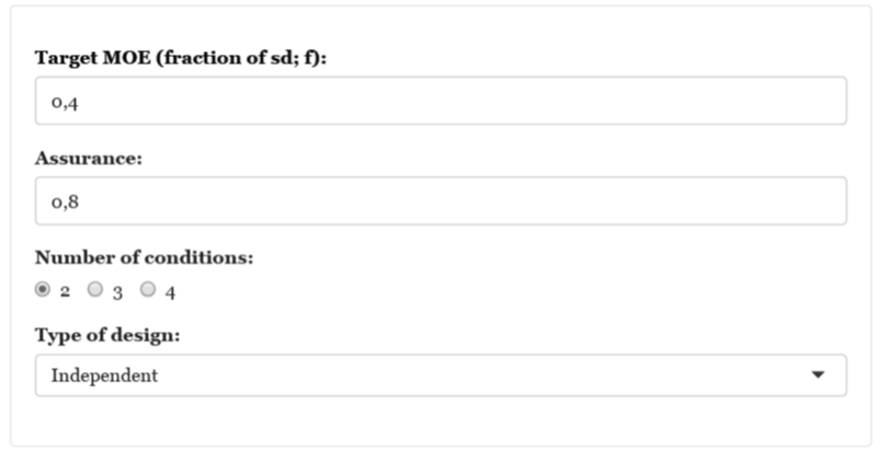
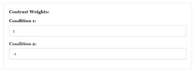
I use the default values (see Figures 1 and 2). And click the “Get Sample size ” button.
Figure 1. Values for Target MoE, assurance and design
Figure 2: Standard contrasts for comparison of two conditions

The output is as follows:

The results give you the sample size for each condition (n), and information about target MoE (f), assurance (assu), the number of conditions (k), and the cross-condition correlation (cor; the value is zero, as it should be in the independent design). With n = 55, there is a 80% probability that f will not be larger than .40.

If you use 55 participants per group the expected MoE equals 0.38.

Of course, using 55 participants per group, makes the total sample size equal to 110.

The output also included a plot of the expected results (what you can expect to happen on average). See Figure 3.

Figure 3: Expected results using n = 55 participants per group in the two groups independent design

This output helps you to consider whether the Expected MoE is small enough. Suppose, for instance, that true difference equals .5 standard deviations, i.e. a medium effect. The figure shows that the expected contrast estimate is a medium effect, and the confidence interval shows that on average values ranging from small to large effects [.12, .88] will be included in the interval. If the difference between small, medium and large effects is important, an expected precision of f = .38 may not be enough, although small and large effects are at the limits of the confidence interval.

A four groups dependent design 

Technical Note:
The app assumes that the sum of squares of the Error Variance can be decomposed in (k – 1) equal parts, where k is the number of conditions. I will change this restriction in a future version of the app. For a custom contrast it is assumed that the contrast is part of an orthogonal set.

Suppose your major interest is the comparison between the average of two groups and the average of two other groups. You have a dependent (repeated measures) design in which participants will be exposed to each of the four treatment conditions. Let’s plan for a target MoE of f = 0.25, with 80 % assurance and let’s suppose our cross-condition correlation equals r = .70. I choose a custom contrast with weights {1/2, 1/2, -1/2, -1/2} (see Figure 4).

Figure 4. Input for sample size planning

The output is as follows.

So, we need 26 participants to have 80% assurance that obtained MoE will not be larger than f = 0.25. Expected MoE is equal to .22. According to the guidelines above, this is a precise estimate.

If you choose “Helmert Contrasts” instead, and press the button without changing anything, the output is as follows.

Under Expected Moe you will see for each of the three contrasts c1, c2, and c3, the weights and expected MOE. The 46 participants give an expected MoE smaller than target MoE, for the least precise estimate (c3; the pairwise comparison) the other expected MoE’s are smaller than that. The Expected Results Figure will display the results for the contrasts with the largest expected MoE.


The new statistics: a five-day course

Last week, I taught a 5-day-course for the LOT (Landelijke Onderzoeksschool Taalwetenschap; Netherlands National Graduate School of Linguistics; www.lotschool.nl) introducing the new statistics to PhD-students working in linguistics and related fields of research. Links to the course materials can be found in this post (apologies for the many typos).

The day-to-day program was as  follows.

  1. Important concepts underlying statistics, like population paremeters, sampling, sanpling distribution, standard error and the margin of error. The primary means of developing these concepts was working with ESCI (www.tiny.cc/itns). The lab assignments are primarily based on Cumming and Calin-Jageman’s (2017) “Introduction to the new statistics”.  The lab-assignments can be found here: www.tiny.cc/newstats. A pdf-version of the presentation can be found here: http://tiny.cc/newstats-presentation
  2. Continuation of day 1. For students that finished the first assignment and to accommodate differences in backgrounds, new lab assignments focusing on statistical assumptions underlying the crucial concepts. Some of these assignments are based on Cumming and Calin-Jageman (2017) and ESCI, others work with R. The lab-assignments can be found here:  www.tiny.cc/newstatsla2
  3. Lecture only. In the lecture we reviewed the basic concepts discovered in the first two days. The concept of a confidence interval was introduced and the p-value. Furthermore, we discussed  NHST by considering (at a procedural level and not so much on a statistical/philosophical level) how the procedure relates to its foundations: Fisher’s significance testing and Neyman and Pearson Hypothesis Testing. We basically saw that NHST is inconsistent with both of these foundations. We also discussed misinterpretations of p-values. The presentation can be found here: www.tiny.cc/newstatsday3. I also made available the lecture notes: www.tiny.cc/newstatsday3ln.
  4. Lecture only. This day was about effect sizes. We considered the unstandardized difference between means,  Cohen’s d, and the case level effect size measures Cohen’s U3 and the Common Language Effectsize. The powerpoint presentation is at www.tiny.cc/newstatsday4.
  5. On the last day the students worked on new lab assignments focusing on interpretations of significance, the use of p-values and effect sizes in published work and working with effect size measures based on SPSS ANOVA output. These assignments can be found here: www.tiny.cc/newstatsday5.