sample size Archives - The small S scientist

April 14, 2019October 22, 2019

Planning for Precise Contrast Estimates: Introduction and Tutorial (Preprint)

I just finished a preprint of an introduction and tutorial to sample size planning for precision of contrast estimates. The tutorial focuses on single factor between and within subjects designs, and mixed factorial designs with one within and one between factor. The tutorial contains R-code for sample size planning in these designs.

The preprint is availabe on researchgate: Click (but I am just as happy to send it to you if you like; just let me know).

March 22, 2019October 22, 2019

Planning with assurance, with assurance

Planning for precision requires that we choose a target Margin of Error (MoE; see this post for an introduction to the basic concepts) and a value for assurance, the probability that MoE will not exceed our target MoE. What your exact target MoE will be depends on your research goals, of course.

Cumming and Calin-Jageman (2017, p. 277) propose a strategy for determining target MoE. You can use this strategy if your research goal is to provide strong evidence that the effect size is non-zero. The strategy is to divide the expected value of the difference by two, and to use that result as your target MoE.

Let’s restrict our attention to the comparison of two means. If the expected difference between the two means is Cohens’s d = .80, the proposed strategy is to set your target MoE at f = .40, which means that your target MoE is set at .40 standard deviations. If you plan for this value of target MoE with 80% assurance, the recommended sample size is n = 55 participants per group. These results are guaranteed to be true, if it is known for a fact that Cohen’s d is .80 and all statistical assumptions apply.

But it is generally not known for a fact that Cohen’s d has a particular value and so we need to answer a non-trivial question: what effect size can we reasonably expect? And, how can we have assurance that the MoE will not exceed half the unknown true effect size? One of the many options we have for answering this question is to conduct a pilot study, estimate the plausible values of the effect size and use these values for sample size planning. I will describe a strategy that basically mirrors the sample size planning for power approach described by Anderson, Kelley, and Maxwell (2017).

The procedure is as follows. In order to plan with approximately 80% assurance, estimate on the basis of your pilot the 80% confidence interval for the population effect size and use half the value of the lower limit for sample size planning with 90% assurance. This will give you 81% assurance that assurance MoE is no larger than half the unknown true effect size.

The logic of planning with assurance, with assurance

There are two “problems” we need to consider when estimating the true effect size. The first problem is that there is at least 50% probability of obtaining an overestimate of the true effect size. If that happens, and we take the point estimate of the effect size as input for sample size planning, what we “believe” to be a sample size sufficient for 80% assurance will be a sample size that has less than 80% assurance at least 50% of the times. So, using the point estimate gives assurance MoE for the unknown effect size with less than 50% assurance.

To make it more concrete: suppose the true effect equals .80, and we use n = 25 participants in both groups of the pilot study, the probability is approximately 50% that the point estimate is above .80. This implies, of course, that we will plan for a value of f > .40, approximately 50% of the times, and so the sample we get will only give us 80% assurance 50% of the times.

The second problem is that the small sample sizes we normally use for pilot studies may give highly imprecise estimates. For instance, with n = 25 participants per group, the expected MoE is f = 0.5687. So, even if we accept 50% assurance, it is highly likely that the point estimate is rather imprecise.

Since we are considering a pilot study, one of the obvious solutions, increasing the sample size so that expected MoE is likely to be small, is not really an option. But what we can do is to use an estimate that is unlikely to be an overestimate of the true effect size. In particular, we can use as our estimate the lower limit of a confidence interval for the effect size.

Let me explain, by considering the 80% CI of the effect size estimate. From basic theory it follows that the “true” value of the effect size will be smaller than the lower limit of the 80% confidence interval with probability equal to 10%. That is, if we calculate a huge number of 80% confidence intervals, each time on the basis of new random samples from the population, the true value of the effect size will be below the lower limit in 10% of the cases. This also means that the lower limit of the interval has 90% probability to not overestimate the true effect size.

This means that if we take the lower limit of the 80% CI of the pilot estimate as input for our sample size calculations, and if we plan with assurance of .90, we will have 90%*90% = 81% assurance that using the sample size we get from our calculations will have MoE no larger than half the true effect size. (Note that for 80% CI’s with negative limits you should choose the upper limit).

Sample Size planning based on a pilot study

Student of mine recently did a pilot study. This was a pilot for an experiment investigating the size of the effect of fluency of delivery of a spoken message in a video on Comprehensibility, Persuasiveness and viewers’ Appreciation of the video. The pilot study used two groups of size n = 10, one group watched the fluent video (without ‘eh’) and the other group watched the disfluent video where the speaker used ‘eh’ a lot. The dependent variables were measured on 7-point scales.

Let’s look at the results for the Appreciation variable. The (biased) estimate of Cohen’s d (based on the pooled standard deviation) equals 1.09, 80% CI [0.46, 1.69] (I’ve calculated this using the ci.smd function from the MBESS-package. According to the rules-of-thumb for interpreting Cohen’s d, this can be considered a large effect. (For communication effect studies it can be considered an insanely large effect). However, the CI shows the large imprecision of the result, which is of course what we can expect with sample sizes of n = 10. (Average MoE equals f = 0.95, and according to my rules-of-thumb that is well below what I consider to be borderline precise).

If we use the lower limit of the interval (d = 0.46), sample size planning with 90% assurance for half that effect (f = 0.23) gives us a sample size equal to n = 162. (Technical note: I planned for the half-width of the standardized CI of the unstandardized effect size, not for the CI of the standardized effect size; I used my Shiny App for planning assuming an independent groups design with two groups). As explained, since we used the lower limit of the 80% CI of the pilot and used 90% assurance in planning the sample size, the assurance that MoE will not exceed half the unknown true effect size equals 81%.

December 22, 2018October 22, 2019

Planning for precise contrast estimates in between subjects designs

Here I would like to explain the procedure for sample size planning for one-way and two-way (factorial) between subjects designs. We will consider examples based on and described in Haans (2018).

The first example: one-way design

The first example considers the effect of seating location of students on their educational performance. Seating location is defined as distance from the teacher and operationalized in terms of the row the student is seated in, with first row being the closest to the teacher and the fourth row being the furthest away. 20 Students are randomly assigned to one of the four possible rows, so N = 20, n = 5. The dependent variable is the course grade of the student. (Note: the data and study are hypothetical).

As Haans (2018) explains, one psychological theory explaining the effect of seating position on educational performance is based on social influence. This theory posits that due to the social influence of the teacher, the students that are seated closest to the teacher find themselves in a state of undivided attention. This undivided attention causes their educational performance to be better than the students who are seated further away.

In operational terms, then, we may expect that first row students will have a better average grade than students seated on the other rows. So, the quantitative research question we are interested in is:

“How much do the average grades differ between students seated first row and the students seated on other rows?”

We can estimate this quantity with a Helmert Contrast, where we assign a contrast weight of 1 to mean of the first row grades and weights -1/3 to the means of the grades in the other rows.

Haans (2018) gives us the following results. The contrast estimate equals 2.00 , 95% CI [0.27, 3.73]. In order to interpret this more easily, we divide this estimate by the square root Mean Square Error, to obtain the standardized estimate and standardized confidence interval (not to be confused with the confidence interval of the standardized estimate, but that’s a different story. The result is: 1.26, 95% CI [0.17, 2.36].

To answer the research question, the estimated difference equals 1.26 standard deviations, which according to rule-of-thumbs frequently used in psychology is a large difference. The CI shows the enormous amount of uncertainty of this estimate: population values between 0.17 (small) and 2.36 (very large) are also consistent with the observed data and our statistical assumptions. So, it seems safe to conclude that it looks like there is a positive effect of seating position, but the wide range of the CI makes it clear that the data do not tell us enough about the size of the effect, the precision is simply too low.

The precision is f = 1.09, which according to my rules-of-thumb is very imprecise (I consider f = 0.65, to be barely tolerable).

So, let’s plan for a replication study with a reasonably precise estimate of f = 0.40, with 80% assurance. (Note: for some advice on setting target Moe: Planning with assurance, with assurance. ) I’ve used the app: https://gmulder.shinyapps.io/PlanningFactorialContrasts/ with the default values for a single factor between subjects design with 4 conditions. According to the app, we need n = 36 participants per condition (making a total of N = 144).

(For more detailed information considering sample size planning for contrast analysis see: http://small-s.science/?p=10 and for some guidelines for setting target MoE: http://small-s.science/?p=14)

The second example: factorial design

Our second example is also taken from Haans (2018). It considered the same phenomenon, the effect of students’ seating distance from the teacher and the educational performance of the students.

A second theory explaining the effect is that the effect is mainly caused by the teacher having decreased levels of eye contact with the students sitting farther to the back in the lecture hall.

To test that theory, a experiment was conducted with N = 72 participants attending a lecture. The lecture was given to two independent groups of 36 pariticpant. The first group attended the lecture while the teacher was wearing dark sunglasses, the second group attented the lecture while the teacher was not wearing sunglasses,. Again, all participants were randomly assigned to 1 of 4 possible rows. The dependent variable was the score on a 10-item questionnaire about the contents of the lecture.

Now, if the eyecontact of the teachter is the causal variable, we may expect that in this experimental setup the difference between the average score of the persons seated on the first row and the averages of the other rows will be smaller for the condition where the teacher wears sunglasses than for the condition in which the teacher does not wear these glasses, as wearing sunglasses prevents eye-contact between the teacher and the students. Our quantitative question is therefore:

“How much does the contrast between the first row and the others rows differ between the conditions with and without sunglasses?”

In other words, we are interested in the size of the interaction effect.

I’ve downloaded the dataset from http://pareonline.net/sup/v23n9.zip (between2by4data.sav) and specified the following syntax in SPSS:

UNIANOVA retention BY sunglasses location
/LMATRIX = “Interaction contrast” sunglasses*location 1 -1/3 -1/3 – 1/3 -1 1/3 1/3 1/3 intercept 0
/DESIGN= sunglasses*location.

The result of the analysis is that the contrast estimate equals 1.0, 95% CI [-0.33, 2.33]. If we standardize this with the within condition variance (the condition being the combination of the levels of the two factors), we get 0.82, 95% CI [-0.27, 1.90].

So, it appears that the difference between the means of the first row and that of the other rows is on average 1.0 points larger in the condition without sunglasses than in the condition with sunglasses. This corresponds to a large difference (d_with = .82). However, the CI also contains negative population difference (albeit that they are smallish), so even though the results are promising for the theory (eyecontact), these negative effects will not persuade a critical reviewer of the study. Indeed, these negative effects contradict the substantive hypothesis.

Again, the confidence interval is so wide, that effects ranging from small negative effects to huge positive effects are considered plausible. Since the results are promising for the theory, a replication study with more precision may be needed to persuade the critics. Let’s plan for a precision of f = .25 with 95% assurance.

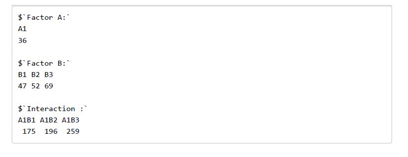
I’ve used the app: https://gmulder.shinyapps.io/PlanningFactorialContrasts/ specifying that we have a factorial design with a = 2 levels and b = 4 levels. The result is that for the interaction contrast with f = .25 and assurance = .95, we need 175 participants per combination of the two factors. This means, that a total of N = 1400 must be recruited.

I’ve taken this from the following output.

Planning for precision of a contrast estimate

Figure 1: Output of sample size planning

I’ve looked at the “Contrast Summary Tab” to check that interaction A1B1 is the correct one (see Figure 2).

Figure 2. Summary of contrast weights.

What’s important in the above figure is that the set of weights for A1B1 matches the set of weights used to get the contrast estimate in SPSS (In the LMATRIX-subcommand), so that’s how we know that A1B1 is the contrast we want. (Note: if you switch the number of levels in the app, that is, use 4 levels for A and 2 for B, the interaction weights will match perfectly).

Reference
Haans, Antal (2018). Contrast Analysis: A Tutorial. Practical Assessment, Research, & Education, 23(9). Available online: http://pareonline.net/getvn.asp?v=23&n=9

October 9, 2017November 7, 2019

Planning for a precise slope estimate in simple regression

In this post, I will show you a way of determining a sample size for obtaining a precise estimate of the slope $\beta_1$ of the simple linear regression equation $\hat{Y_i} = \beta_0 + \beta_1X_i$ . The basic ingredients we need for sample size planning are a measure of the precision, a way to determine the quantiles of the sampling distribution of our measure of precision, and a way to calculate sample sizes.

As our measure of precision we choose the Margin of Error (MOE), which is the half-width of the 95% confidence interval of our estimate (see: Cumming, 2012; Cumming & Calin-Jageman, 2017; see also www.thenewstatistics.com).

The distribution of the margin of error of the regression slope

In the case of simple linear regression, assuming normality and homogeneity of variance, MOE is $t_{.975}\sigma_{\hat{\beta_1}}$ , where $t_{.975}$ , is the .975 quantile of the central t-distribution with $N - 2$ degrees of freedom, and $\sigma_{\hat{\beta_1}}$ is the standard error of the estimate of $\beta_1$ .

An expression of the squared standard error of the estimate of $\beta_1$ is $\frac{\sigma^2_{Y|X}}{\sum{(X_i - \bar{X})}^2}$ (Wilcox, 2017): the variance of Y given X divided by the sum of squared errors of X. The variance $\sigma^2_{Y|X}$ equals $\sigma^2_y(1 - \rho^2_{YX})$ , the variance of Y multiplied by 1 minus the squared population correlation between Y and X, and it is estimated with the residual variance $\frac{\sum{(Y -\hat{Y})^2}}{df_e}$ , where $df_e = N - 2$ .

The estimated squared standard error is given in (1)

(1) $\hat{\sigma}_{\hat{\beta_{1}}}^{2}=\frac{\sum(Y-\hat{Y})^{2}/df_{e}}{\sum(X-\bar{X})^{2}}.$

With respect to the sampling distribution of MOE, we first note the following. The distribution of estimates of the residual variance in the numerator of (1) is a scaled $\chi^2$ -distribution:

$\frac{\sum(Y-\hat{Y})^{2}}{\sigma_{y}^{2}(1-\rho^{2})}\sim\chi^{2}(df_{e}),$

thus

$\frac{\sum(Y-\hat{Y})^{2}}{df_{e}}\sim\frac{\sigma_{y}^{2}(1-\rho^{2})\chi^{2}(df_{e})}{df_{e}}.$

Second, we note that

$\frac{\sum(X-\bar{X})^{2}}{\sigma_{X}^{2}}\sim\chi^{2}(df),$

where $df = N - 1$ , therefore

$\sum(X-\bar{X})^{2}\sim\sigma_{X}^{2}\chi^{2}(df).$

Alternatively, since $\sum{(X - \bar{X})^2} = df\sigma^2_X$ , and multiplying by 1 ( $\frac{df}{df}$ ).

$df\sigma_{X}^{2}\sim df\sigma_{X}^{2}\chi^{2}(df)/df.$

In terms of the sampling distribution of (1), then, we have the ratio of two (scaled) $\chi^2$ distributions, one with $df_e = N - 2$ degrees of freedom, and one with $df = N - 1$ degrees of freedom. Or something like:

$\hat{\sigma}_{\hat{\beta_{1}}}^{2}\sim\frac{\sigma_{y}^{2}(1-\rho^{2})\chi^{2}(df_{e})/df_{e}}{df\sigma_{X}^{2}\chi^{2}(df)/df}=\frac{\sigma_{y}^{2}(1-\rho^{2})}{df\sigma_{X}^{2}}\frac{\chi^{2}(df_{e})/df_{e}}{\chi^{2}(df)/df}=\frac{\sigma_{y}^{2}(1-\rho^{2})F(df_{e,}df)}{df\sigma_{X}^{2}},$

which means that the sampling distribution of MOE is:

(2) $\hat{MOE}\sim t_{.975}(N-2)\sqrt{\frac{\sigma_{y}^{2}(1-\rho^{2})F(N-2,N-1)}{(N-1)\sigma_{X}^{2}}}.$

This last equation, that is (2), can be used to obtain quantiles of the sampling distribution of MOE, which enables us to determine assurance MOE, that is the value of MOE that under repeated sampling will not exceed a target value with a given probability. For instance, if we want to know the .80 quantile of estimates of MOE, that is, assurance is .80, we determine the .80 quantile of the (central) F-distribution with N – 2 and N – 1 degrees of freedom and fill in (2) to obtain a value of MOE that will not be exceeded in 80% of replication experiments.

For instance, suppose $\sigma^2_Y = 1$ , $\sigma^2_X = 1$ , $\rho = .50$ , $N = 100$ , and assurance is .80, then according to (2), 80% of estimated MOEs will not exceed the value given by:

vary = 1
varx = 1
rho = .5
N = 100 
dfe = N - 2
dfx - N - 1
assu = .80
t = qt(.975, dfe)
MOE.80 = t*sqrt(vary*(1 - rho^2)*qf(.80, dfe, dfx)/(dfx*varx))
MOE.80

## [1] 0.1880535

What does a quick simulation study tell us?

A quick simulation study may be used to check whether this is at all accurate. And, yes, the estimated quantile from the simulation study is pretty close to what we would expect based on (2). If you run the code below, the estimate equals 0.1878628.

library(MASS)
set.seed(355)
m = c(0, 0)

# note: s below is the variance-covariance matrix. In this case,
# rho and the cov(y, x) have the same values
# otherwise: rho = cov(x, y)/sqrt(varY*VarX) (to be used in the 
# functions that calculate MOE)
# equivalently, cov(x, y) = rho*sqrt(varY*varX) (to be used
# in the specification of the variance-covariance matrix for 
#generating bivariate normal variates)

s = matrix(c(1, .5, .5, 1), 2, 2)
se <- rep(10000, 0)
for (i in 1:10000) {
theData <- mvrnorm(100, m, s)
mod <- lm(theData[,1] ~ theData[,2])
se[i] <- summary(mod)$coefficients[4]
}
MOE = qt(.975, 98)*se
quantile(MOE, .80)

##       80% 
## 0.1878628

Planning for precision

If we want to plan for precision we can do the following. We start by making a function that calculates the assurance quantile of the sampling distribution of MOE described in (2). Then we formulate a squared cost function, which we will optimize for the sample sizeusing the optimize function in R.

Suppose we want to plan for a target MOE of .10 with 80% assurance.We may do the following.

vary = 1
varx = 1
rho = .5
assu = .80
tMOE = .10

MOE.assu = function(n, vary, varx, rho, assu) {
        varY.X = vary*(1 - rho^2)
        dfe = n - 2
        dfx = n - 1
        t = qt(.975, dfe)
        q.assu = qf(assu, dfe, dfx)
        MOE = t*sqrt(varY.X*q.assu/(dfx * varx))
        return(MOE)
}

cost = function(x, tMOE) { 
cost = (MOE.assu(x, vary=vary, varx=varx, rho=rho, assu=assu) 
- tMOE)^2
}

#note samplesize is at least 40, at most 5000. 
#note that since we already know that N = 100 is not enough
#in stead of 40 we might just as well set N = 100 at the lower
#limit of the interval
(samplesize = ceiling(optimize(cost, interval=c(40, 5000), 
tMOE = tMOE)$minimum))

## [1] 321

#check the result: 
MOE.assu(samplesize, vary, varx, rho, assu)

## [1] 0.09984381

Let’s simulate with the proposed sample size

Let’s check it with a simulation study. The value of estimated .80 of estimates of MOE is 0.1007269 (if you run the below code with random seed 335), which is pretty close to what we would expect based on (2).

set.seed(355)
m = c(0, 0)

# note: s below is the variance-covariance matrix. In this case,
# rho and the cov(y, x) have the same values
# otherwise: rho = cov(x, y)/sqrt(varY*VarX) (to be used in the 
# functions that calculate MOE)
# equivalently, cov(x, y) = rho*sqrt(varY*varX) (to be used
# in the specification of the variance-covariance matrix for 
# generating bivariate normal variates)

s = matrix(c(1, .5, .5, 1), 2, 2)
se <- rep(10000, 0)
samplesize = 321
for (i in 1:10000) {
theData <- mvrnorm(samplesize, m, s)
mod <- lm(theData[,1] ~ theData[,2])
se[i] <- summary(mod)$coefficients[4]
}
MOE = qt(.975, 98)*se
quantile(MOE, .80)

##       80% 
## 0.1007269

References

Cumming, G. (2012). Understanding the New Statistics. Effect Sizes, Confidence Intervals, and Meta-Analysis. New York: Routledge
Cumming, G., & Calin-Jageman, R. (2017). Introduction to the New Statistics: Estimation, Open Science, and Beyond. New York: Routledge.
Wilcox, R. (2017). Understanding and Applying Basic Statistical Methods using R. Hoboken, New Jersey: John Wiley and Sons.