This is a short tutorial on comparing two means with the independent and paired t-test in jamovi.
Description of the data
I have downloaded the dataset from the Mathematics and Statistics Help (MASH) site. The dataset contains data on 78 persons following one of three diets. I will use the dataset to show you how to estimate the difference between two means with the independent t-test analysis and the dependent t-test analysis in jamovi. I will ignore the different diets and focus on gender differences and pre- and post-weight differences instead.
I will focus on two substantive research questions.
- To what extent does following a diet lead to weight loss?
- To what extent does the weight lost differ between females and males?
The paired t-test in jamovi
Let’s start with the first research question. Statistical analysis can be useful for answering the research question, but then we will first have to translate the substantive question into a statistical one. Now, it seems reasonable to assume that if following a diet leads to weight loss, that the typical weight before the diet differs from the typical weight after following the diet. If we assume furthermore that the mean provides a good representation of what is typical, then it is plausible that the mean weight before the diet differs from the mean weight after the diet.
If we are interested in the extent to which means differ, we are – statistically speaking – interested in the extent to which expected values differ. So, our analysis will focus on finding out what our data have to say about the difference between the expected values. More concrete: we focus on the difference between the expected values for weight (measured in kg) before and after the diet. Using conventional symbols, we aim at uncovering quantitative information about the difference \mu_{pre\ weight} – \mu_{post\ weight}.
Since all persons were measured pre and post diet, the measurements are likely to be correlated. Indeed, the sample correlation equals r = .96. We need to take this correlation into account and that is why we use the statistical techniques for estimation and testing that are available in the paired t-test analysis in jamovi.
Doing the paired t-test in jamovi
In a real research situation, we would of course start with descriptive analyses to figure out what the data seem to suggest about the extent to which a diet leads to weight loss. But now we are just looking at how to obtain the relevant inferential information from jamovi.
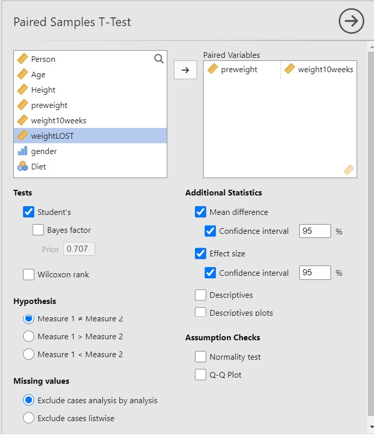
I have chosen the following options for the analysis.

Since we are interested in the extent to which following a diet leads to weight loss, it is important to realize that the t-test in itself does not necessarily provide useful information. Why? Because the t-test gives us input to make the decision whether to reject the null-hypothesis that the expected values are equal, and only indirectly provides us with the information about the extent to which the expected values differ, and the latter is of course what we are interested in: we want quantitative information! The more useful information is provided by the estimate of the mean difference and the 95% Confidence Interval.
The paired t-test output
The relevant output for the t-test and the estimation results are presented in Figure 2.

Let’s start with the t-test. The conventional null-hypothesis is that the expected values of the two variables are equal ( \mu_{pre\ weight} = \mu_{post\ weight}, or \mu_{pre\ weight} – \mu_{post\ weight} = 0. . The alternative hypothesis is that the expected values are not equal. Following convention, we use a significance level of \alpha = .05, so that our decision rule is to reject the null-hypothesis if the p-value is smaller than .05 and to not reject but also not accept the null-hypothesis if the p-value is .05 or larger.
The result of the t-test is t(77) = 13.3, p < .001. Since the p-value is smaller than .05 we reject the null-hypothesis and we decide that the expected values are not equal. In other words, we decide that the population means are not equal. As we said above, this does not answer our research question, so we’d better move on to the estimation results.
The estimated difference between the expected values equals 3.84 kg, 95% CI [3.27, 4.42]. So, we estimate that the difference in expected weights after 10 weeks of following the diet is somewhere between 3.72 and 4.42 kilograms.
Cohen’s d for the paired design
Jamovi also provides point and interval estimates for Cohen’s d. This version of Cohen’s d is derived by standardizing the mean difference using the standard deviation of the difference scores. Figure 3 presents the relevant output. The estimated value of Cohen’s delta equals 1.51, 95% CI [1.18, 1.83]. Using rules of thumb for the interpretation of Cohen’s d, these results suggest that there may be a very large difference in mean weights of the pre- and postdiet measurements.

There is an alternative conceptualisation of the standardized mean difference. Instead of using the SD of the difference scores, we may use the average of the SDs of the two measurements. See https://small-s.science/2020/12/cohens-d-for-paired-designs/ for an explanation and R-code for the calculation of the CI.
The independent t-test in jamovi
To answer the second research question, we will have to reframe the substantive question into a statistical one. Just like we assumed above, we will consider the difference between the expected values (or population means) to be the statistical quantity of interest.
The conventional statistical null-hypothesis of the t-test is that the expected value of the variable does not differ between the groups or conditions. In other words, the null-hypothesis is that the two population means are equal. If the test result is significant, we will reject the null-hypothesis and decide that the population means are not equal. Note that this does not really answer the research question. Indeed, we are interested in the extent to which the expected values differ and not in whether we can decide that the difference is not zero. For that reason, estimation results are usually more informative than the results of a significance test.
Doing the independent t-test in jamovi.
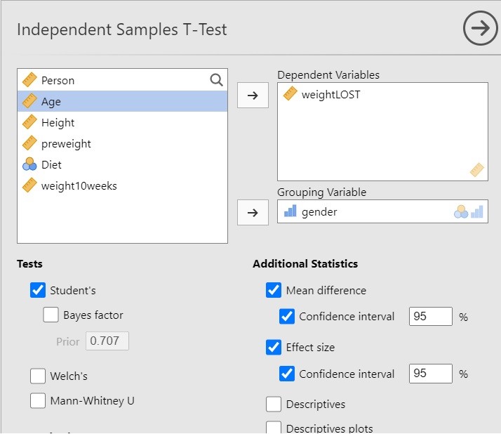
I have chosen the following options for the independent t-test analysis in jamovi.

The above options will give you the results of the independent t-test and, more importantly, the estimation results, both unstandardized and standardized (Cohen’s d).
The independent t-test output
The relevant output is presented in Figure 5.

The result of the t-test is t(74) = -0.21, p = 0.84. This test result is clearly not significant, so we cannot decide that the population means differ. Importantly, we can also not decide that the population means are equal. That would be an instance of accepting the null-hypothesis and that is not allowed in NHST.
The estimation results (i.e. -0.12 kg, 95% CI [-1.29, 1.04]) make it clear that we should not necessarly believe that the population means are equal. Indeed, even though the estimated difference is only 0.12 kilograms, the CI shows the data to be consistent with differences up to 1 kg in either direction, i.e. with women showing more average weight loss than men or women showing less average weight loss than men.
Cohen’s d for the independent design
We can also find the standardized mean difference and its CI in the independent t-test output: Cohen’s d = -0.08, 95% CI [-0.50, 0.41]. In this case, Cohen’s d is based on the pooled standard deviaton. According to rules-of-thumb that are used frequently in psychology the estimated effect is negligible to small, but the CI shows the data to be consistent with medium effect sizes in either direction.


